6. Tutorials
This section provides a few tutorials to get a user started in CanFlood. It is suggested to work through the tutorials sequentially, referring to Section5 when more detailed information is desired. For all tutorials, the project CRS can safely be set from any of the data layers, unless otherwise specified. Tutorials are written assuming users are familiar with QGIS and object-based flood risk modelling. All tutorial data can be found in the latest ‘tutorial_data’ zip on the project page.
6.1. Tutorial 1a: Risk (L1)
This tutorial guides the user through the simplest application of risk modelling in CanFlood, called a level 1 (L1) analysis, where only binary exposure is calculated. This ‘exposed vs. not exposed’ analysis can be useful for preliminary analysis where there is insufficient information to model more complex object vulnerability.
6.1.1. Load data to the project
Download the data layers for Tutorial 1:
haz_rast: hazard event rasters with WSL value predictions for the study area for four probabilities.
o haz_0050.tif
o haz_0100.tif
o haz_0200.tif
o haz_1000.tif
finv_tut1a.gpkg : flood asset inventory (’finv’) spatial layer.
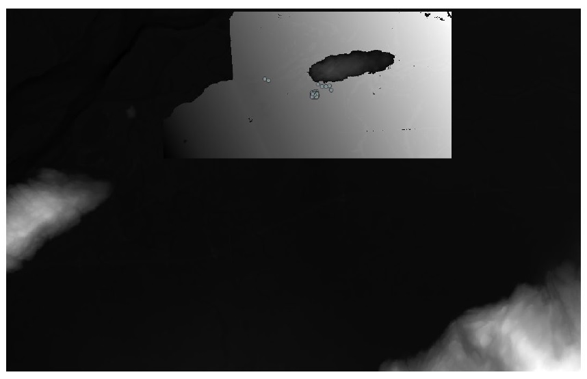
Ensure your project’s CRS is set to ‘EPSG:3005’ (Depending on your settings, this may have been set automatically when you loaded the datafiles. All tutorials use CRS ‘EPSG:3005’ unless stated otherwise. See the following link for an explanation of projections in QGIS. https://docs.qgis.org/3.10/en/docs/user_manual/working_with_projections/working_with_projections.html ) and load the downloaded layers into a new QGIS project (Depending on your QGIS settings, you may be requested to select a transformation if the CRS was not set correctly beforehand). Your map canvas should look something like this:
Explore the flood asset inventory (‘finv’) layer’s attributes (F6). You should see something like this:
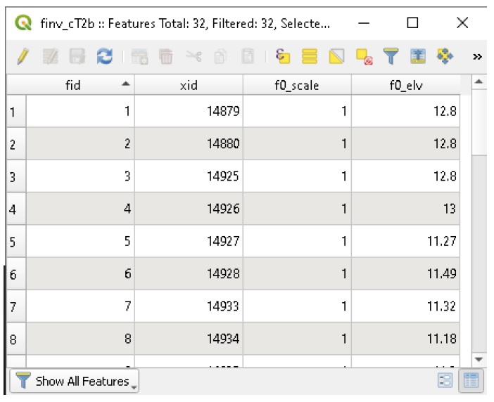
The 4 fields are:
fid: built-in feature identifier (not used);
xid: Index FieldName, unique identifier for the asset (Any field with unique integer values can be used as the FieldName Index (except built-in feature identifiers));
f0_scale: value to scale the results of the ‘f0’ calculation for this asset;
f0_elv: height (above the project datum) at which the asset is vulnerable to flooding.
For this example, each inventory entry or ‘asset’ could represent a home with the main floor elevation entered into ‘f0_elv’. Any flood waters above this elevation will be tabulated as an impact for that asset. For CanFlood’s L1 analysis, based on the user supplied likelihood of each event, the total ‘risk of inundation’ for each asset and for the full study area will be computed.
6.1.2. Build the Model
Press the ‘Build’ button  to begin building a CanFlood model.
Setup
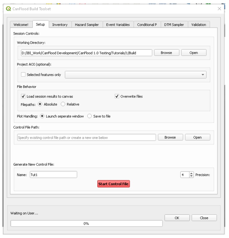
On the ‘Setup’ tab, configure your ‘Build Session’ by first creating or selecting an easy to locate working directory using the ‘Browse’ button. CanFlood will place all the data files assembled with the ‘Build’ toolset in this directory. Ensure the remaining ‘Build Controls’ are specified as shown below.
Now use the lower portion of the dialog to specify the parameters CanFlood should use to assemble your new Control File as shown below.
Once the parameters are correctly entered, click ‘Start Control File’ to create your Control File in the working directory. There should be a message on the QGIS Toolbar indicating the process ran successfully.
If you view the ‘CanFlood’ Log Messages Tab (View > Panels > Log Messages), you can see the log messages for the process you just completed. It should look something like this:
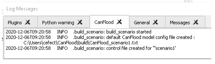
Back in CanFlood’s ‘Setup’ tab, next to the working directory file path, click ‘Open’ to open the specified working directory, you should see the Control File ‘CanFlood_Tut1.txt’ created in your working directory. Open the control file. This is a template with some blank, default, and specified parameters. As you work through the remainder of ‘Build’ section of this tutorial, blank parameters will be filled in by the CanFlood tools. Notice the ‘#’ comment letting you know how and when this control file was created. ‘#’ comment lines are ignored by the program when reading from the control file, and are written by some tools to help the user track actions taken by CanFlood on the control file.
Store Inventory
Move to the ‘Inventory’ tab. Under the Inventory Compiler section, select the inventory layer (finv_tut1a) and ensure ‘elevation type’ is set to ‘datum’ to reflect that the inventory’s ‘f0_elv’ values are measured from the project’s datum (rather than ground). Now select the inventory vector layer and the appropriate ‘Index FieldName’ as shown, then click ‘Store’.
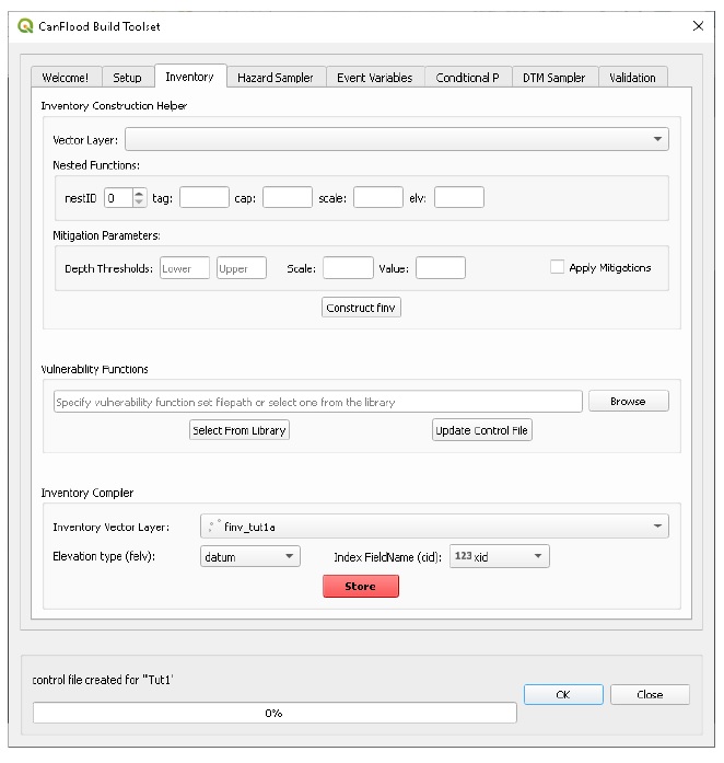
You should see the inventory csv file stored into the working directory. This is a simplified version of the inventory layer with the spatial data removed. Open the Control File again. You should notice that asset inventory (‘finv’) parameter has been populated with the file name of the newly created csv.
Hazard Sampler
Move to the ‘Hazard Sampler’ tab. Check all the hazard rasters in the display box as shown (If the hazard layers are not shown in the dialog, hit ‘Refresh’), leaving the remaining parameters blank or untouched:
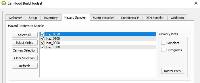
Click ‘Sample Rasters’ to generate the exposure (‘expos’) dataset. You should see a new csv file in the working directory, and its filepath added to the control file under ‘expos’. These are the WSLs sampled at each asset from each hazard event raster.
Event Variables
Now that the WSLs have been stored, we need to tell CanFlood what the probability of realizing each of these events is. Move to the ‘Event Variables’ tab. Specify the correct values for each event’s likelihood (from the event names) as shown:
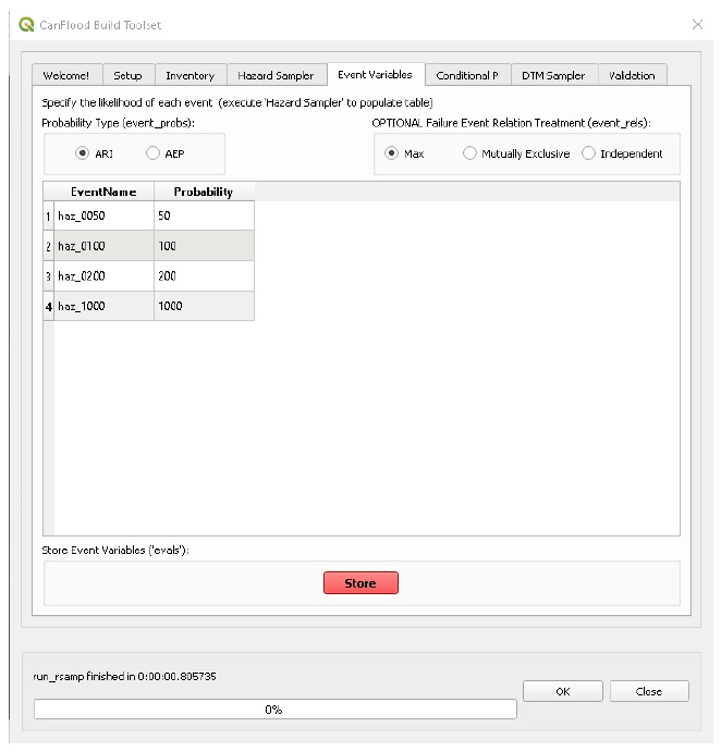
Press ‘Store’. The event probabilities (‘evals’) dataset should have been created and its filepath written to the Control File under ‘evals’.
Validation
Move to the ‘Validation’ tab, check ‘Risk (L1)’, then click ‘Validate’. This will check all the inputs in the control file and set the ‘risk1’ validation flag to ‘True’ in the control file. Without this flag, the CanFlood model will fail.
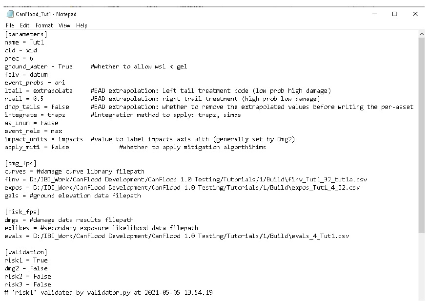
The control file should now be fully built for an L1 analysis and the necessary inputs assembled. The completed control file should look similar to this (but with your directories):
6.1.3. Run the Model
Click the ‘Model’ button  to launch the Model toolset dialog.
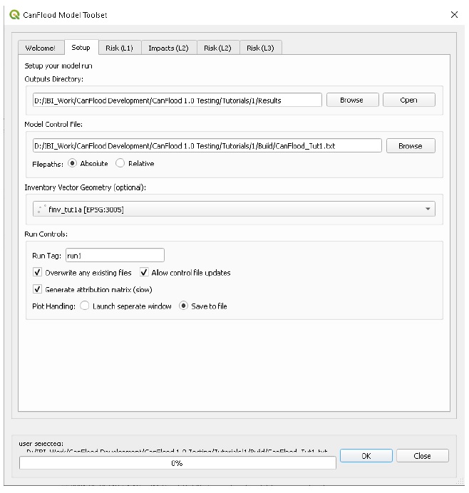
Setup
On the ‘Setup’ tab, select a working directory (does not have to match the directory from the previous step) where all your results will be stored. Also select your control file created in the previous section if necessary.
Your dialog should look like this (CanFlood will attempt to automatically identify the Inventory Vector Layer; however, this tutorial does not make use of this layer so the selection here can be ignored):
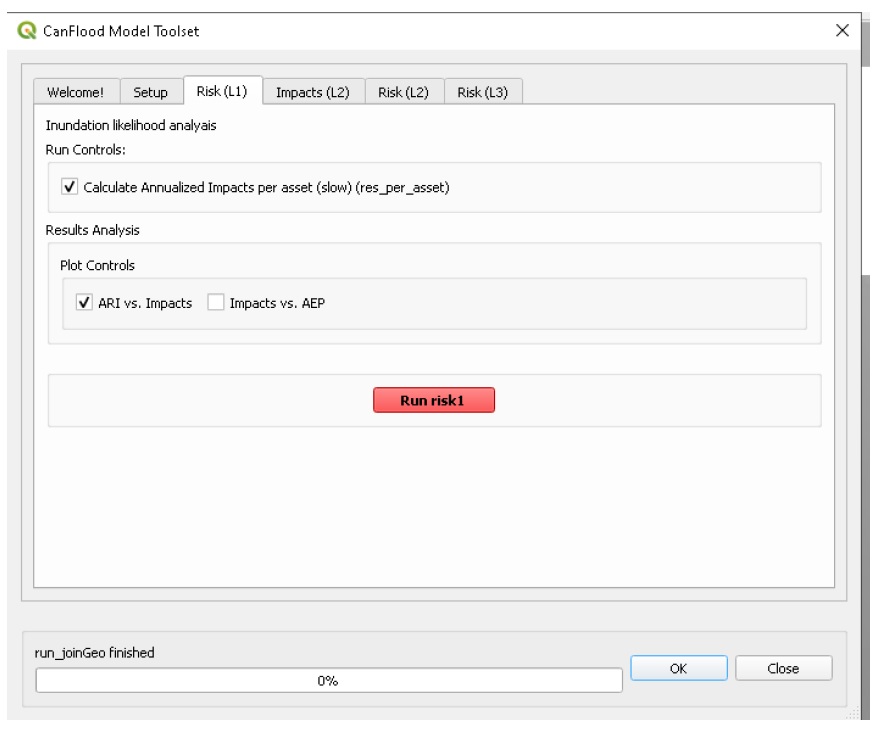
Execute
Navigate to the ‘Risk (L1)’ tab. Check the first two boxes as shown below and press ‘Run risk1’:
6.1.4. View Results
Navigate to the selected working directory. You should see 3 files created:
risk1_run1_tut1a_passet.csv: expected value of inundation per asset;
risk1_run1_tut1a_ttl.csv: total results, expected value of total inundation per event (and for all events);
tut1a.run1 Impact-ARI plot on 6 events.svg: a plot of the total results (see below).
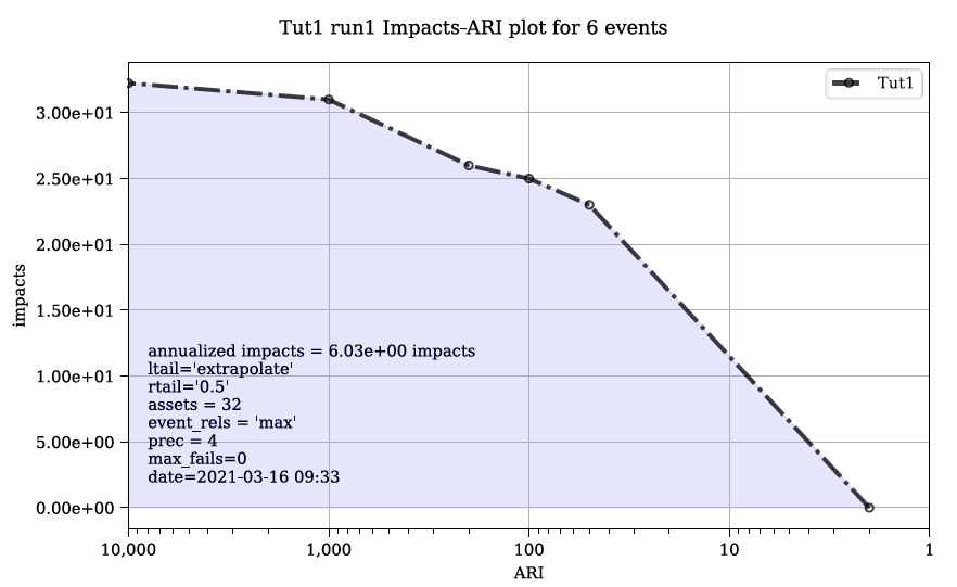
These are the non-spatial results which are directly generated by CanFlood’s model routines. To facilitate more detailed analysis and visualization, CanFlood comes with a third and final ‘Results’ toolset.
Join Geometry
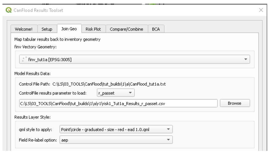
Open the results toolset by clicking the ‘Results’  button. The CanFlood models are designed to run independent of the QGIS spatial API. Therefore, if you would like to view the results spatially, additional actions are required to re-attach the tabular model results to the asset inventory (‘finv’) vector geometry. To do this, move to the ‘Join Geo’ tab, select the asset inventory (‘finv’) layer. Then select ‘r_passet’ under ‘results parameter to load’ to populate the field below with a filepath to your per-asset results file (If the filepath fails to populate automatically, try changing re-setting the ‘finv’ and ‘parameter’ drop-downs. Alternatively, enter the filepath manually). Finally, select the ‘Results Layer Style’ and ‘Field re-label option’ as shown:
Click ‘Join’. A new temporary ‘djoin’ layer should have been loaded onto the map canvas with the selected style applied. Move this layer to the top of your layers panel and turn off the original ‘finv’ layer to see the new ‘djoin’ layer. The ‘djoin’ layer should be a points layer where the size of each point is relative to the magnitude of the expected value of inundation (i.e. the average number of inundations per year) similar to this:
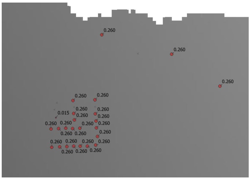
Open the attributes table for the ‘djoin’ layer (F6). You should something similar to the below table:
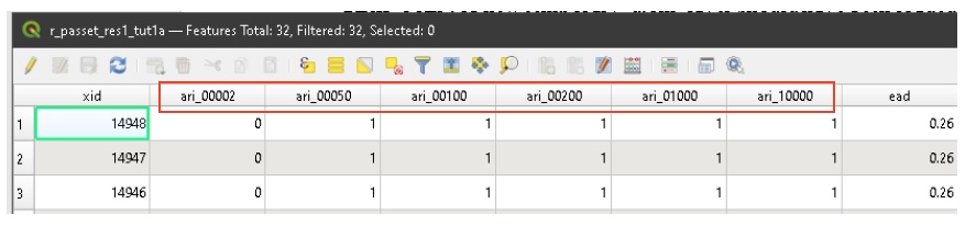
Notice the six impact fields (boxed in red above) have had their names converted to ‘ari_probability’ and the field values provide the binary exposure (0=not exposed; 1=exposed) results. You’ll need to save this layer if you want it to be available in another QGIS session (Layers Pane > Right Click the layer > Save As…). Congratulations on your first CanFlood run!
6.2. Tutorial 2a: Risk (L2) with Simple Events
Tutorial 2 demonstrates the use of CanFlood’s ‘Risk (L2)’model (Section5.2.3). This emulates a more detailed risk assessment where the vulnerability of each asset is known and described as a function of flood depth (rather than simple binary flood presence as in tutorial 1). This tutorial also demonstrates an inventory with ‘relative’ heights and CanFlood’s ‘composite vulnerability function’ feature where multiple functions are applied to the same asset.
6.2.1. Load data to project
Download the tutorial 2 data from the ‘tutorials2data’ folder:
haz_rast: hazard event rasters with WSL value predictions for the study area for four probabilities.
o haz_0050.tif
o haz_0100.tif
o haz_0200.tif
o haz_1000.tif
finv_tut2.gpkg: flood asset inventory (’finv’) spatial layer
dtm_tut2.tif: digital terrain model raster with ground elevation predictions
haz_frast: companion failure event rasters(not used in tutorial 2a)
haz_fpoly: companion failure event polygons(not used in tutorial 2a)
Load these into a QGIS project, it should look something like this:
6.2.2. Build the Model
Open the ‘Build’ toolset.
Scenario Setup
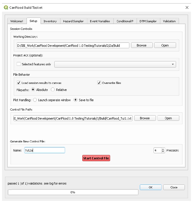
On the ‘Setup’ tab, configure the session as shown using your own paths, then click ‘Start Control File’:
Select Vulnerability Function Set
Move to the ‘Inventory’ tab and click ‘Select From Library’ to launch the library selection GUI shown below. Select the library ‘IBI_2015’ in the top left window then ‘IBI2015_DamageCurves.xls’ in the bottom left window, then click ‘Copy Set’ to copy this set of vulnerability functions into your working directory. The inventory provided in this tutorial has been constructed specifically for these ‘IBI2015’ functions. Generally, flood risk modellers must develop or supply their own vulnerability functions.
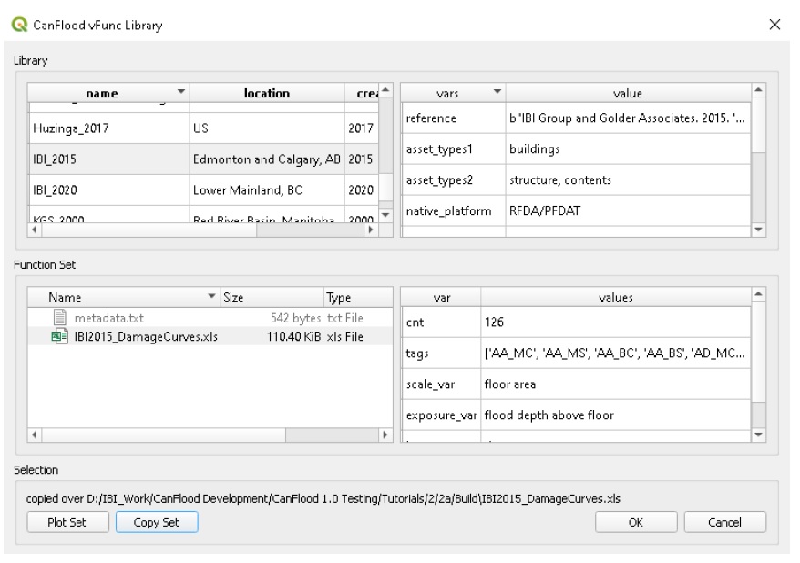
Close the ‘vFunc Selection’ GUI, and you should now see the new .xls file path entered under ‘Vulnerability Functions’. Finally, click ‘Update Control File’ to store a reference to this vulnerability function set into the control file.
Inventory
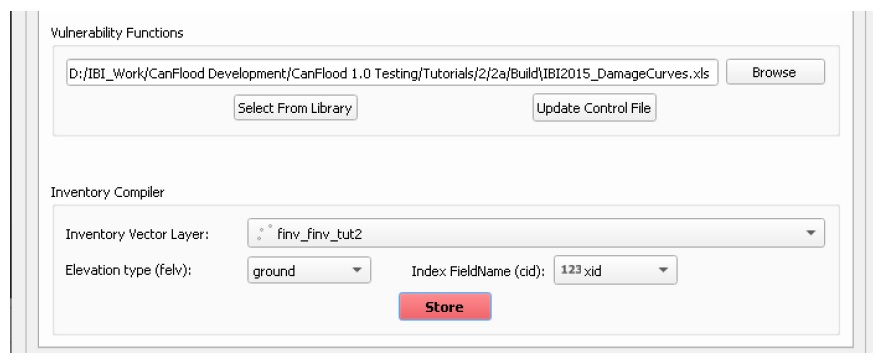
On the same ‘Inventory’ tab, select the inventory vector layer, the appropriate Index FieldName, and set the elevation type to ‘ground’ as shown, then click ‘Store’.
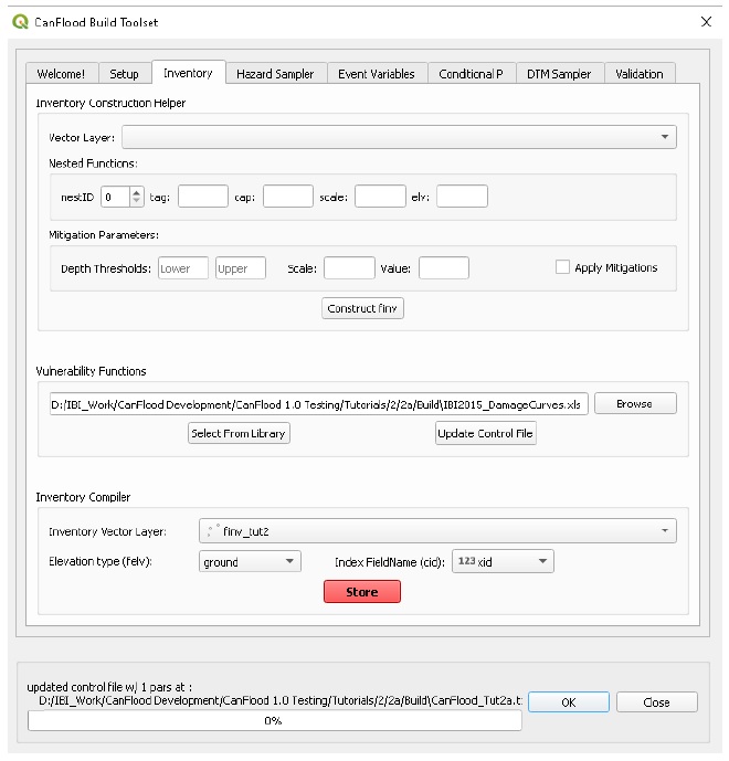
You should see the inventory csv now stored in the working directory.
Hazard Sampler
Move to the ‘Hazard Sampler’ tab, ensure the four hazard rasters are shown in the window and all other fields are default, then click ‘Sample Rasters’. You should see the ‘expos’ data file created in the working directory.
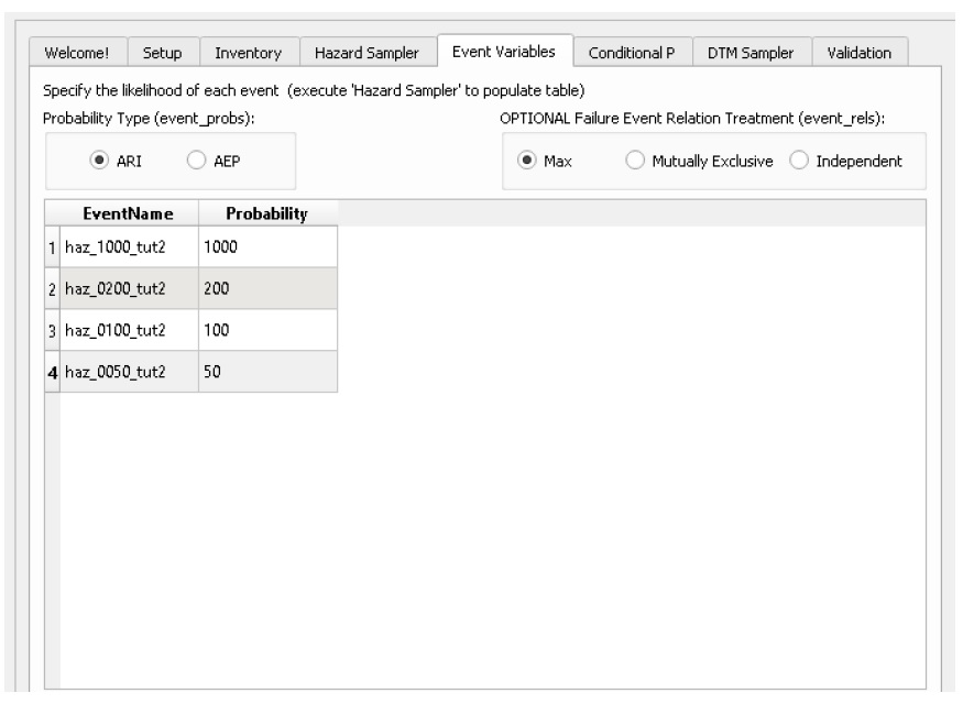
Event Variables
Move to the ‘Event Variables’ tab, you should now see the 4 hazard events from the previous task populating the table. Fill in the ‘Probability’ values as shown (ignore the ‘Failure Event Relation’ setting for now), then click ‘Store’ to generate the event variables (‘evals’) dataset.
DTM Sampler
Move to the ‘DTM Sampler’ tab. Select the ‘dtm_tut2’ raster then click ‘Sample DTM’ to generate the ground elevation (‘gels’) dataset in your working directory and create a reference to it in the Control File.
Validation
Move to the ‘Validation’ tab, check the boxes for both L2 models, then click ‘Validate’. You should get a log message ‘passed 1 (of 2) validations. see log’. To investigate the failed validation attempt, open the Log Messages panel, it should look like this:
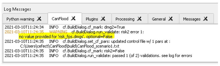
This shows that the Risk (L2) model is missing the ‘dmgs’ data file and will not run. This is expected behavior as CanFlood separates the exposure calculation (Impacts L2) from the risk calculation. We will calculate this ‘dmgs’ data file and validate for Risk (L2) in the next section. You’re now ready to run the Impacts (L2) model!
6.2.3. Run the Model
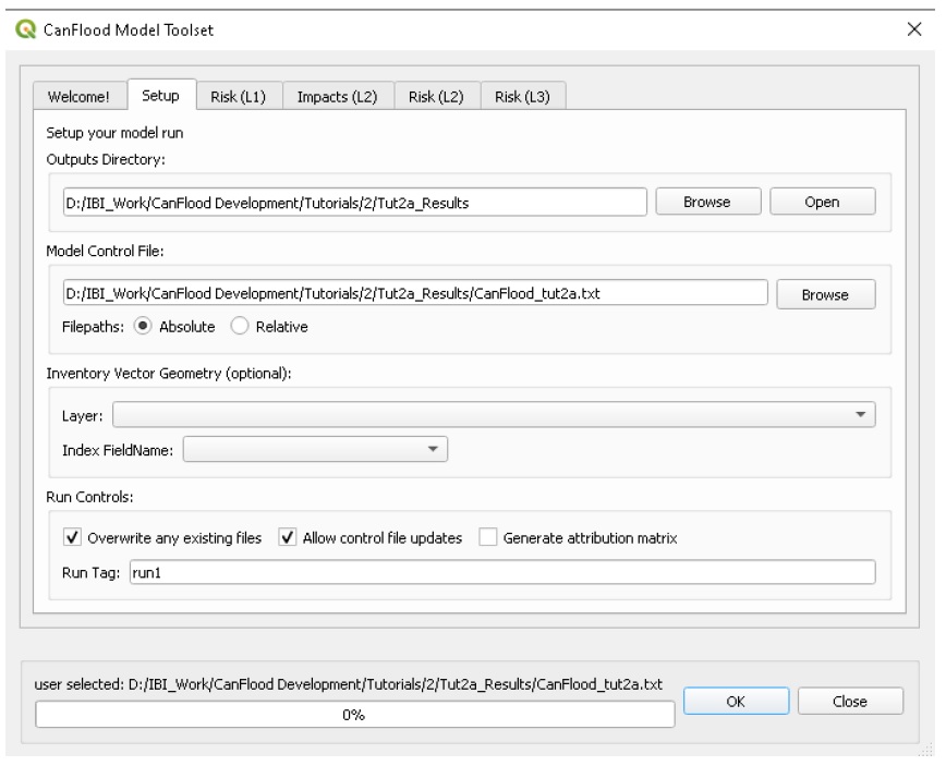
Open the ‘Model’ dialog. Configure the ‘Setup’ tab as shown below, selecting your own paths and control file, and ensuring the ‘Outputs Directory’ is a sub-directory of your previous ‘Working Directory’ (Some ‘Results’ tools work better when the model output data files are in the same file tree as the Control File):
Impact (L2)
Move to the ‘Impacts (L2)’ tab. Ensure the ‘Run Risk (L2)’ box is not checked (we’ll execute the risk model manually in the next step) but that ‘Output expanded component impacts’ is checked. Click ‘Run dmg2’.
This should create an impacts (‘dmgs’) datafile in your working directory and fill in the corresponding entry on the control file. Open this csv. It should look something like this:
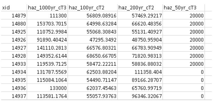
These are the raw impacts per event per asset calculated with each vulnerability function, the sampled WSL and the sampled DTM elevation. The second output is the ‘expanded component impacts’, a large optional output background file used by CanFlood that contains the tabulation of each nested function and the applied scaling and cap values. See Section5.2.2 for more information. Now you’re ready to calculate flood risk!
Risk (L2)
Move to the ‘Risk (L2)’ tab. Check all the boxes shown below and click ‘Run risk2’.
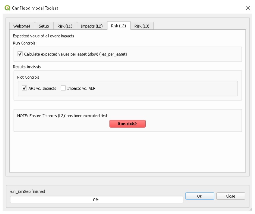
A set of results files should have been generated (discussed below). For a complete description of the Risk (L2) module, see Section5.2.3.
6.2.4. View Results
After completing the Risk (L2) run, navigate to your working directory. It should now contain these files:
eventypes_run1_tut2a.csv: derived parameters for each raster;
risk2_run1_tut2a_r2_passet.csv: expected value per asset expanded Risk (L2) results;
risk2_run1_tut2a_ttl.csv: total expected value of all events and assets Risk (L2) results;
dmgs_tut2a_run1.csv: per asset Impacts (L2) results;
dmgs_expnd_tut2a_run1.csv: expanded component Impacts (L2) results;
run1 Impacts-ARI plot for 6 events.svg: see below.
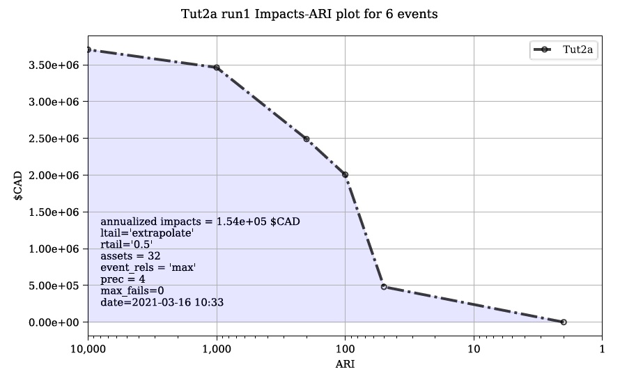
Figure 6-1: Summary risk curve plot of the total Risk (L2) results.
Risk Plots
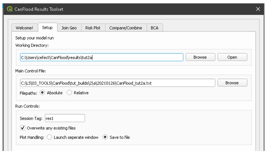
While the Risk modules include some basic risk curve plots (see above), CanFlood provides additional plot customization under the ‘Risk Plot’ tool in the ‘Results’ toolset. Open the ‘Results’ toolset, configure the session by selecting a working directory, the Control File, and setting ‘Plot Handling’ to ‘Save to file’ as shown:
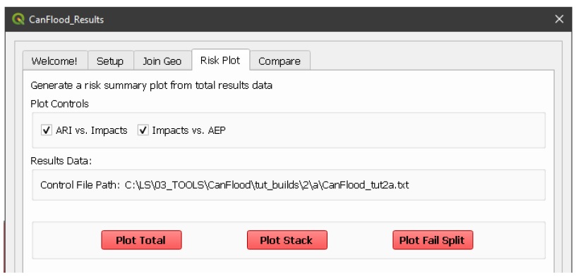
To generate the custom plots, navigate to the ‘Risk Plot’ tab, and select both plot types as shown below:
To customize the plot, open the Control File, and under ‘[plotting]’, change the following parameters:
color = red
impactfmt_str = ,.0f
These parameters control the colour of the plot and the formatting applied to the impact values. Save the changes, then return to the CanFlood window and hit ‘Plot Total’. You should see the two plots below generated in your working directory.
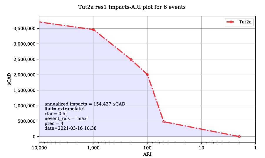
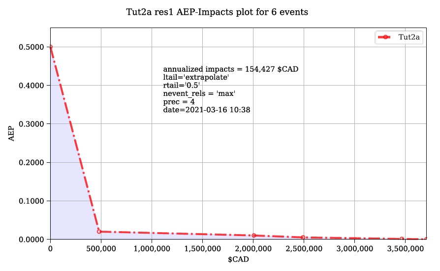
These plots are the two standard risk curve formats for the same total results data. Alternatively, changing ‘Plot Handling’ to ‘Launch separate window’ on the ‘Setup’ tab will launch a dialog window after plotting that provides some built-in tools for further customizing the plot.
6.3. Tutorial 2b: Risk (L2) with Dike Failure
Users should first complete Tutorials 1 and 2a. Tutorial 2b uses the same input data as 2a but expands the analysis to demonstrate the risk analysis of a simple levee failure through incorporating a single companion failure event into the model. This companion failure event is composed of two layers:
haz_1000_fail_A_tut2: ‘failure raster’ indicating the WSL that would be realized were any of the levee segments to fail during the event; and
haz_1000_fail_A_tut2: conditional exposure probability polygon layer with features indicating the extent and probability of failure of each levee segment during the flood event (‘failure polygons’). Notice this layer contains two features that overlap in places, corresponding potential flooding from two breach sites in the levee system. This layer will be used to tell CanFlood when and how to sample the failure raster.
This simplification by using these two layers facilitates the specification of multiple failure probabilities but where any failure (or combination of failures) would realize the same WSL (Section5.1.5’s ‘complex conditionals’). Ensure these layers are loaded into the same QGIS project as was used for Tutorial 2a.
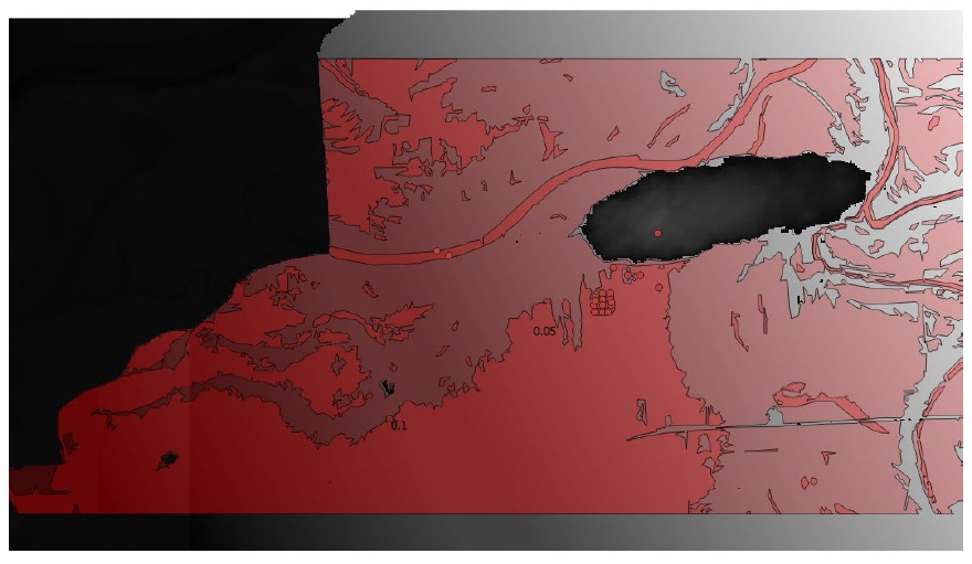
To better understand the ‘failure polygons’ layer, let’s apply CanFlood’s ‘red fill transparent’ style. Begin by loading this style template into your profile with the ‘Add Styles’ tool (Plugins > CanFlood > Add Styles), then apply it using the Layer Styling Panel (F7). Finally, add a single label for ‘p_fail’ and move the layer just beneath the asset inventory (‘finv’) points layer on the layers panel. Your canvas should look similar to the below:
6.3.1. Build the Model
Follow the steps in Tutorials 2a ‘Build the Model’ but with including the ‘failure raster’ (‘haz_1000_fail_A_tut2’, probability=1000ARI) in the ‘Hazard Sampler’ and ‘Event Variables’ steps. On the ‘Event Variables’ step, ensure ‘Failure Event Relation Treatment’ is set to ‘Mutually Exclusive’.
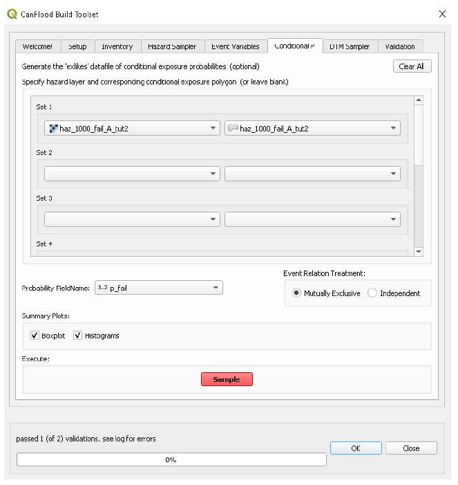
Conditional Probabilities
Navigate to the ‘Conditional P’ tab to resolve the overlapping failure polygons into the resolved exposure probabilities (‘exlikes’) dataset to tell CanFlood what probability should be assigned to each asset when realizing the companion failure raster. Start by pairing the failure polygons with the failure raster, select the ‘Probability FieldName’, ‘Event Relation Treatment’, and ‘Summary Plots’ as shown, then click ‘Sample’:
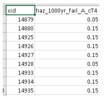
A resolved exposure probabilities (‘exlikes’) data file should have been created in your working directory with entries like this:
Two non-spatial summary plots of this data should also have been generated in your working directory, the most useful for this particular model being the histogram:
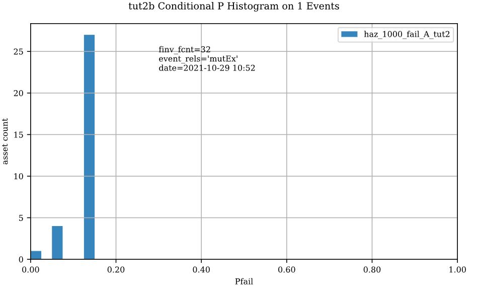
These values are the conditional probabilities of each asset realizing the 1000-year companion failure event WSL(Try running the tool again, but this time selecting ‘Max’. If you look closely at the boxplots, you should see a slight difference in the resolved probabilities. This suggests this model is not very sensitive to the relational assumption of these overlapping failure polygons). See Section5.2.3 for a complete description of this tool. Complete the model construction by running the ‘DTM Sampler’ and ‘Validation’ tools.
6.3.2. Run the Model
Open the ‘Model’ dialog and setup your session similar to Tutorial 2a but ensure ‘Generate attribution matrix’ is checked under ‘Run Controls’ (we’ll use this to make plots showing the different components that contribute to the risk totals).
Impacts and Risk
Navigate to the ‘Impacts (L2)’ tab, check the ‘Run Risk (L2) upon completion’ box to execute the exposure and risk models in sequence from your Control File. Navigate to the ‘Risk (L2)’ tab and ensure ‘Calculate expected values per asset’ is checked. Now move back to the ‘Impacts (L2)’ tab and click ‘Run dmg2’. You should see the same types of outputs as Tutorial 2a, but with two additional ‘attribution matrix’ datasets.
6.3.3. View Results
To better understand the influence of incorporating levee failure, this section will demonstrate how to generate a plot showing the total risk and the portion of that total risk that comes from assuming no failure. Open the ‘Results’ toolset and configure your session by selecting a working directory and the same Control File used above. Now navigate to the ‘Risk Plot’ tab, ensure both plot controls are checked, then click ‘Plot Fail Split’. This should generate two risk plot formulations, including the figure below:
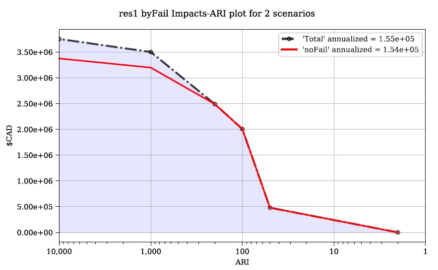
In this plot, the red line represents the contribution to risk without the companion failure events, which should be nearly identical to the results from Tutorial 2a, and a second line showing the total results(Alternatively, the ‘Compare’ tool can be used to generate a comparison plot between the two tutorials). The area between these two lines illustrates the contribution to risk from incorporating levee failure into the model.
6.4. Tutorial 2c: Risk (L2) with Complex Failure
It is recommended that users first complete Tutorial 2b. Tutorial 2c uses the same input data as 2b but expands the analysis to demonstrate the incorporation of more complex levee failure with two companion failure events into the model.
In the same QGIS project as was used for Tutorial 2b, ensure the following are also added to the project:
haz_1000_fail_B_tut2.gpkg: failure polygon ‘B’;
haz_1000_fail_B_tut2.tif: failure raster ‘B’.
These layers represent an additional companion failure event ‘B’ for the 1000-year event where the failure WSL and probabilities are different but complimentary from those of Tutorial 2b’s companion failure event ‘A’. These could be outputs from two modelled breach scenarios.
6.4.1. Build the Model
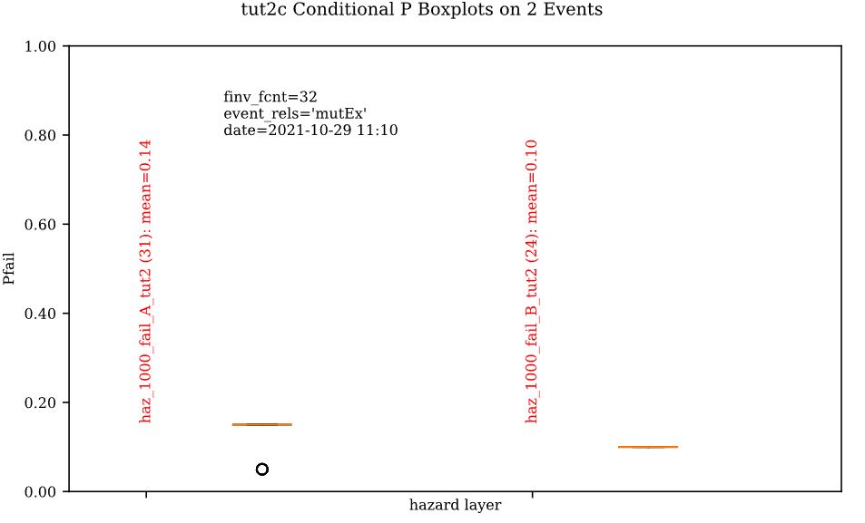
Follow the steps in Tutorials 2b ‘Build the Model’ but with including the additional companion failure event ‘B’ in the ‘Hazard Sampler’, ‘Event Variables’ and ‘Conditional P’ steps. For the latter two, ensure both event relation treatments are set to ‘Mutually Exclusive’. Looking at the ‘Conditional P’ boxplot shows the difference in failure probabilities specified by the two companion failure events:
Complete the model construction by running the ‘DTM Sampler’ and ‘Validation’ tools.
6.4.2. Run the Model
Open the ‘Model’ dialog and follow the steps in Tutorial 2b to setup this model run.
Impacts and Risk
Execute the ‘Impacts (L2)’ and ‘Risk (L2)’ models similar to Tutorial 2b but ensure ‘Generate attribution matrix’ is de-selected.
To explore the influence of the ‘event_rels’ parameter, open the control file, change the ‘event_rels’ parameter to ‘max’, change the ‘name’ parameter to something unique (e.g., ‘tut2c_max’), then save the file with a different name. On the ‘Setup’ tab, point to this modified control file, a new outputs directory, and run both models again as described above (Advanced users could avoid re-running the ‘Impacts (L2)’ model by manipulating the Control File to point to the ‘dmgs’ results from the previous run as these will not change between the two formulations).
6.4.3. View Results
After executing the ‘Risk (L2)’ model for the ‘event_rels=mutEx’ and ‘event_rels=max’ control files, two similar collections of output files should have been generated in the two separate output directories specified during model setup. To visualize the difference between these two model configurations, open the ‘Results’ toolset and select a working directory and the original ‘event_rels=mutEx’ control file as the ‘main control file’ on the ‘Setup’ tab (The control file specified on the ‘Setup’ tab will be used for common plot styles (e.g.,). Before generating the comparison files, configure the plot style by opening the same main control file, and changing the following ‘[plotting]’ parameters:
‘color = red’
‘linestyle = solid’
‘impactfmt_str = ,.0f’
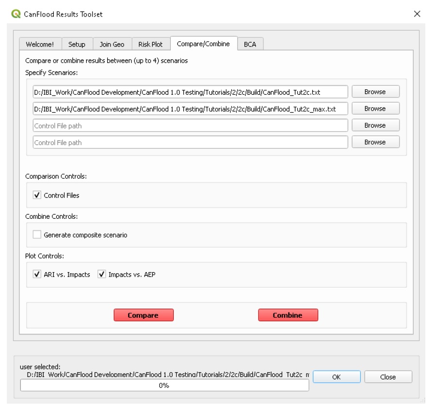
To generate a comparison plot of these two scenarios, navigate to the ‘Compare/Combine’ tab, select the ‘Control File’ for both model configurations generated in the previous step, ensure ‘Control Files’ is checked under ‘Comparison Controls’, as shown below:
Click ‘Compare’ to perform the comparison. You should see two files generated in your working directory:
Comparison plot showing both risk curves on the same axis; and
Control file comparison spreadsheet.
The control file comparison spreadsheet is shown below and is an easy way to quickly identify distinctions between model scenarios.
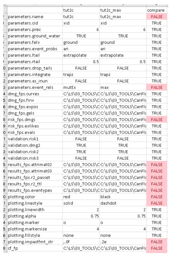
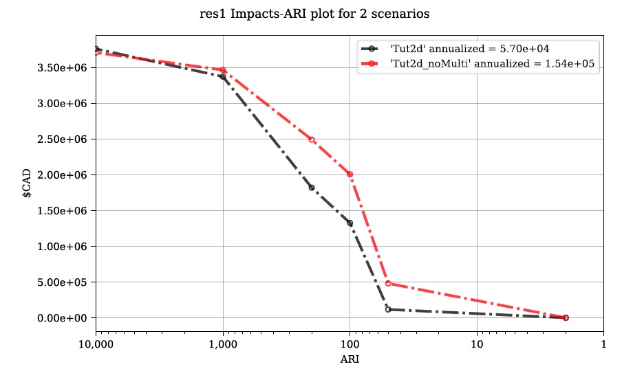
On the comparison plot (shown below), notice the difference in the risk curves and annualized values is negligible, indicating the treatment of event relations is not very significant for this model.
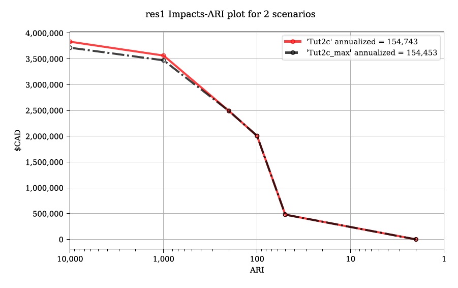
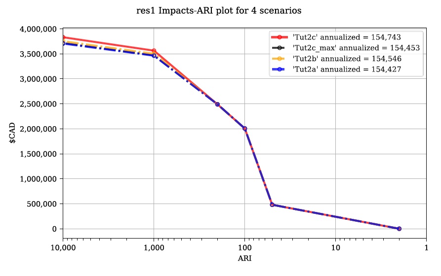
Re-running the comparison tool on the four Tutorial 2 control files constructed thus far yields the following:
6.5. Tutorial 2d: Risk (L2) with Mitigation
It is recommended that users first complete Tutorial 2a before proceeding. Tutorial 2d uses the same input data as 2a but expands the analysis to demonstrate the incorporation of object (or property) level mitigation measures (PLPM) into the model. This can be useful for improving the accuracy of a model where two assets are functionally similar, using the same vulnerability function, but where one has some mechanism to reduce the exposure of the asset (e.g., a backflow valve). Similarly, this functionality can be used to investigate the benefits of introducing PLPMs with a comparative analysis.
6.5.1. Build the Model
Follow the steps in Tutorials 2a ‘Build the Model’, with the exception of the ‘Inventory’ step, which we’ll modify to apply four new fields to the inventory vector layer (‘finv’) by configuring the ‘Inventory’ tab as shown below before clicking ‘Construct finv’:
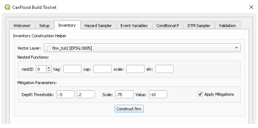
This should create a new layer with a ‘finv’ prefix in your map canvas. Exploring the attribute table of this layer (F6) should show the four new fields that were created and filled with the values specified. These are used by the ‘Impacts (L2)’ module to modify the exposure passed to each objects vulnerability function and are described in Section5.2.2. Complete the inventory construction by ensuring ‘Apply Mitigations’ is checked, the newly created inventory vector layer is selected, and the remainder of the tab is configured as shown below (same as Tutorial 2a). Click ‘Store’.
Complete the ‘Hazard Sampler’, ‘Event Variables’, ‘DTM Sampler’, and ‘Validation’ steps as described in Tutorial 2a.
6.5.2. Run the Model
Open the ‘Model’ dialog and setup your session similar to Tutorial 2a.
Impacts and Risk
Navigate to the ‘Impacts (L2)’ tab and ensure ALL ‘Run Controls’ are checked then click ‘Run dmg2’. You should see the same types of outputs as Tutorial 2a, but with some additional outputs that will help us understand the influence of the mitigation parameters, including the box plot shown below:
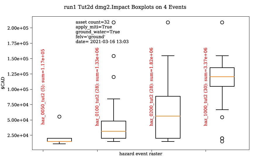
This shows data summaries for the four event rasters, the total impact values (in red text), and some key model info.
To understand the effect of the mitigation parameters, open the control file, change the ‘apply_miti’ parameter to ‘False’, change the ‘name’ parameter to ‘tut2d_noMiti’, ‘color’ to ‘red’, and save it under a different name. On the ‘Setup’ tab, point to this new control file and change the ‘Run Tag’ to ‘noMiti’. Now move back to the ‘Impacts (L2)’ tab and click ‘Run dmg2’ again. You should see another boxplot generated in your working directory:
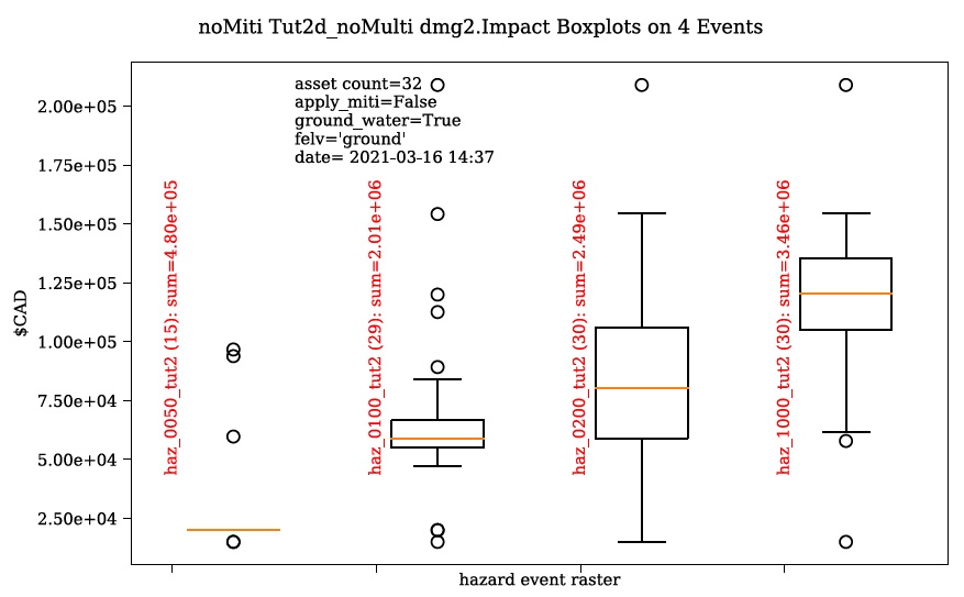
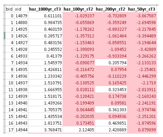
Notice the smaller events (50yr and 100yr) have changed significantly, while the larger events less-so. This makes sense considering we told CanFlood the mitigations would be overwhelmed at depths above 0.2 m (via the upper depth threshold parameter). We can investigate this model behavior further by opening either (The influence of the mitigation functions on the depths are not reflected in this output) of the ‘depths_’ outputs, which should look similar to the below (values below the upper threshold are highlighted in red for clarity):
Similarly, the ‘dmg2_smry’ spreadsheet ‘_smry’ tab for the mitigation run shows the change in total impact values (per event) calculated at each step of the ‘Impacts (L2)’ module (bars and arrow added for clarity):
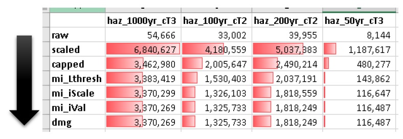
This shows the total impacts achieved by the raw curves, then the ‘scaling’ algorithm (‘fX_scale’) the ‘capping’ algorithm (‘fX_cap’), followed by the algorithm that enforced the lower threshold (‘mi_Lthresh’), the mitigation scaling (‘mi_iScale’), the mitigation value addition (‘mi_iVal’), and the final result (identical to the previous row). This progression shows that the ‘capping’ algorithm had a large influence on the results and the mitigation value addition (‘mi_iVal’) had negligible influence.
6.5.3. View the Results
The ‘Compare’ Results tool can be used to show the influence on the risk curve and total risk:
6.6. Tutorial 2e: Benefit-Cost Analysis
This tutorial demonstrates CanFlood’s Benefit-Cost Analysis (BCA) tools for supporting basic benefit-cost analysis for flood risk interventions like the mitigations considered in the previous tutorial. Before continuing with this tutorial, users should have completed and have available the results data for Tutorial 2a (Alternatively, the ‘tut2d_noMiti’ from Tutorial 2d can be used) and 2d:
CanFlood_tut2a.txt: control file from Tutorial 2a with valid total results (‘r_ttl’) file and filepath;
CanFlood_tut2d.txt: control file from Tutorial 2d with valid total results (‘r_ttl’) file filepath.
Begin by opening the ‘Results’ toolbox then navigating to the ‘Setup’ tab to configure it using the control file from Tutorial 2d. Now we’ll generate a test plot to make sure our control files are valid. Ensure the ‘impactfmt_str’ parameter is set to ‘,.0f’ (no apostrophes) in the Tutorial 2d control file. Now move to the ‘Compare/Combine’ tab, enter in both control files, check one of the ‘Plot Controls’, then click ‘Compare’. A plot identical to the one generated at the end of Tutorial 2d should have been generated. Note the EAD of Tutorial 2d is ~57,000. This is the residual annual flood risk for these assets, after the PLPM intervention.
Complete BCA Workbook
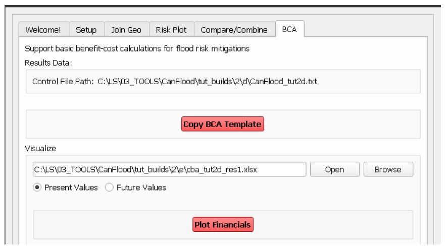
Navigate to the ‘BCA’ tab. Ensure the control file path for Tutorial 2d is shown at the top of the window, then click ‘Copy BCA Template’. You should see a new ‘cba_xls’ parameter set in the control file and your ‘BCA’ window should look similar to the below:
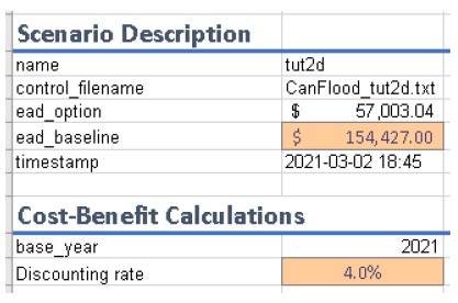
Now click ‘Open’ to edit the BCA workbook. You should see the ‘smry’ tab populated with information from Tutorial 2d, most notably the $57k EAD calculated for this option. Complete the remaining input cells on the ‘smry’ tab by specifying the EAD from 2a and a 4% discounting rate as shown below:
Now move to the ‘data’ tab on the workbook to enter in the benefit-cost data of pursuing the Tutorial 2d mitigations. For this tutorial, assume we have determined the following for this intervention:
Installation of the PLPMs will take 2 years at $1M/year and provide protection for 100 years;
Maintenance will cost $1k/year beginning once construction completes and continue for the 100-year lifecycle of the intervention;
There will be no change in relative benefits or maintenance costs over time.
The two EAD rows on the ‘data’ tab should be automatically populated based on the values specified on the ‘smry’ tab; however, to match the assumptions above we must adjust some of these values as shown in the first six-years of the ‘data’ tab:
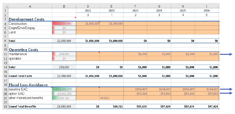
Notice the first year of the ‘baseline’ and ‘option’ EAD are blank, reflecting that no benefits are gained yet; however, the second year shows half the benefits will be realized. The $1000/year maintenance costs should extend through the full 100 years (i.e., copy/paste onto all rightward cells — not shown).
Once the ‘data’ tab is complete, a ‘B/C ratio’ of 1.18 should be shown on the ‘smry’ tab (If you get a B/C ratio of 1.19, make sure the $1000 maintenance costs are entered for every year of the life-cycle). Save and close this spreadsheet.
Plot Financials
To further summarize and analyze the data entered into the BCA worksheet (make sure to hit save!), move back to the CanFlood ‘BCA’ window, select ‘Future Values’, and click ‘Plot Financials’. The plot shown below should be generated:
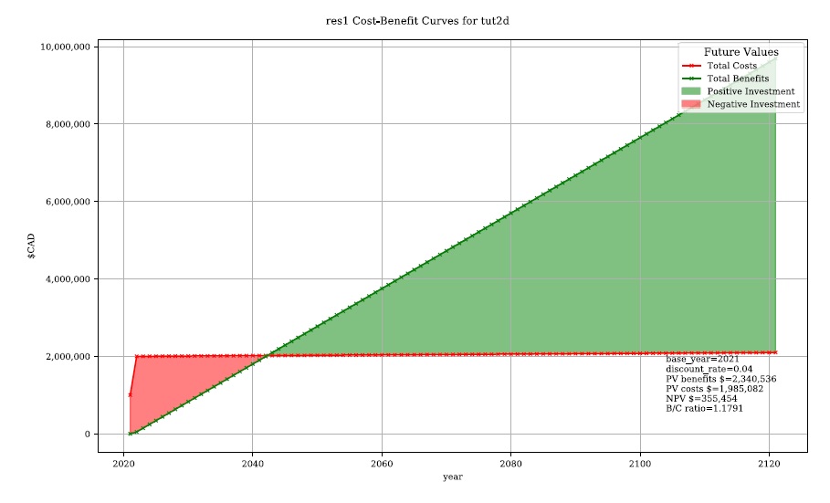
This shows the relative values of the cumulative benefits and costs over time (without discounting). Notice the expensive installation costs exceed the benefits initially; however, after ~25 years the benefits of this option outweigh the costs (the ‘pay-back year’). Also notice that, with future values, the plot shows cumulative benefits around $10M at 100 years. Perhaps by then we will all be living in spaceships… so maybe it’s best not to consider such far-off benefits of flood mitigation so significantly.
Change the radio button to ‘Present Values’ and click ‘Plot Financials’ again. You should see a plot like the below:
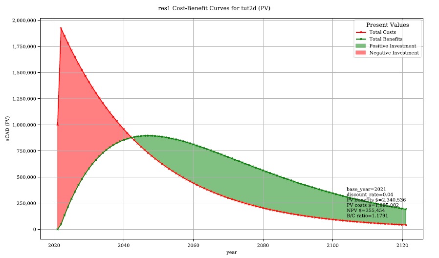
Notice the ‘B/C ratio’ and the ‘pay-back year’ have not changed, but the plot now shows the costs and benefits decaying with time, reflecting the application of the discount rate.
To better understand the role of the discount rate, return to the worksheet, change the discount rate to 8%, save the worksheet, and in the CanFlood window click ‘Plot Financials’ again:
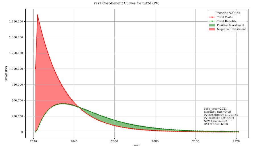
Notice the ‘payback year’ has not changed, but the relative size of the positive (green) and negative (red) areas has shifted and the ‘B/C ratio’ has dropped below 1. This reflects the more severe discounting of the future benefits brought by the larger 8% discount rate. In other words, by the time the future residents of the study area accrue significant benefits from the PLPMs, the current stakeholders wish they had spent the money on something else.
6.8. Tutorial 4a: Risk (L1) with Percent Inundation (Polygons)
This tutorial demonstrates a risk analysis of polygon type assets where the impact metric is percent inundated rather than depth. This can be useful for some coarse risk modelling, or for assets like agricultural fields where the loss can reasonably be calculated from the percent of the asset that is inundated.
Load the following data layers from the ‘tutorials4data’ folder:
haz_rast: hazard event rasters with WSL value predictions for the study area for four probabilities.
o haz_0050_tut4.tif
o haz_0100_tut4.tif
o haz_0200_tut4.tif
o haz_1000_tut4.tif
dtm_cT2.tif: DTM layer (and corresponding stylized layer definition .qlr file)
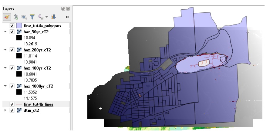
finv_tut4a_polygons.gpkg: flood asset inventory (’finv’) spatial layer
finv_tut4b_lines.gpkg:(used in tutorial 4b)
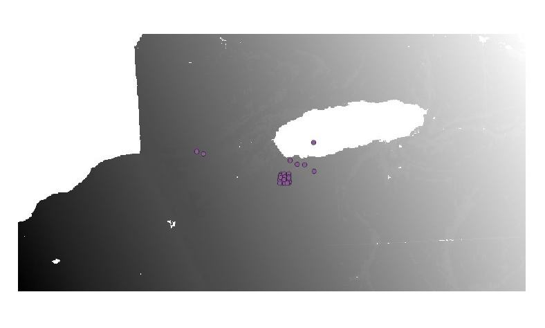
Move the polygon inventory (‘finv’) layer to the top, apply the CanFlood ‘fill transparent blue’ style (Available in the CanFlood styles package described in Section5.4.4 (Plugins > CanFlood > Add Styles)), and your project should look similar to this (Be sure to load the stylized ‘.qlr’ layers in place of the raw layers):
6.8.1. Build the Model
Setup
Launch the CanFlood ‘Build’ toolset and navigate to the ‘Setup’ tab. Set the ‘Precision’ field (This is important for inundation percent analysis which deals with small fractions) to ‘6’, then complete the typical setup as instructed in Tutorial 1a.
Inventory
Navigate to the ‘Inventory’ tab, ensure ‘Elevation type’ is set to ‘datum’ (Risk (L1) inundation percentage runs can not use asset elevations; therefore, this input variable is redundant. When as_inun=True CanFlood model routines expect an ‘elv’ column with all zeros) then click ‘Store’.
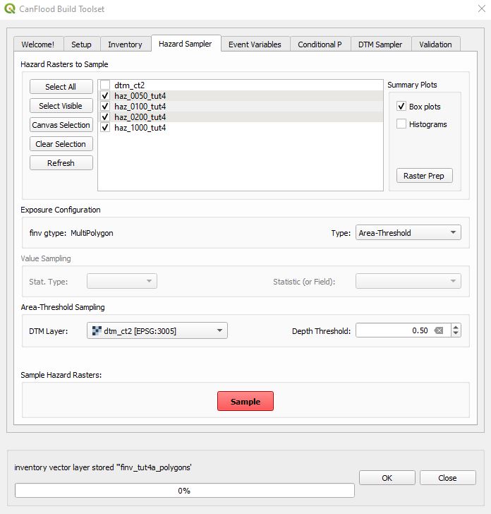
Hazard Sampler
Navigate to the ‘Hazard Sampler’ tool, load the four hazard rasters into the dialog window, check ‘Box plots’, under Exposure Configuration select ‘Area-Threshold’ as the type, set the ‘Depth Threshold’ to 0.5, and select the DTM layer as shown:
Click ‘Sample Rasters’. Navigate to the exposure data file (‘expos’) this created in your working directory. You should see a table like this:
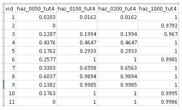
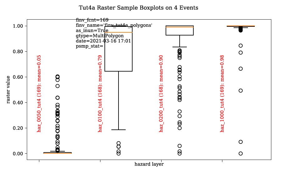
These values are the calculated percent of each polygon with inundation greater than the specified depth threshold (0.5m). The generated box plots show this data graphically:
Event Variables and Validation
Run the ‘Event Variables’ and ‘Validation’ tools as instructed in Tutorial 1a.
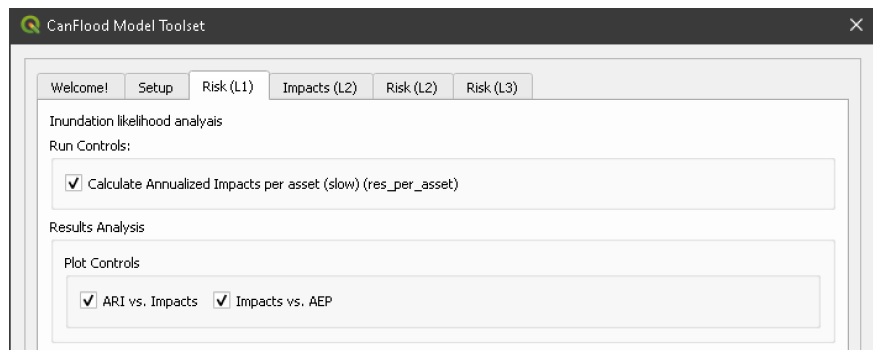
6.8.2. Run the Model
Open the ‘Model’ dialog and follow the steps in Tutorial 1a to setup this model run. Navigate to the ‘Risk (L1)’ tool, check the boxes shown, and click ‘Run risk1’:
The set of results files discussed below should have been generated.
6.8.3. View the Results
Navigate to your working directory. You should see the following results files have been generated:
risk1_run1_tut4_passet.csv: per asset results
risk1_run1_tut4_ttl.csv
tut4a run1 AEP-Impacts plot for 6 events.svg
tut4a run1 Impacts-ARI plot for 6 events.svg
Open the per-asset results (‘passet’) data file, it should look like this:
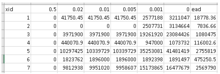
The first non-index columns are simply the inundation percentage (from the ‘expos’ data file) multiplied by the asset scale attribute (from the ‘finv’ data file). The final ‘ead’ column is the expected value of these four columns.
To visualize this, open the ‘Results’ toolbox and configure the ‘Setup’ tab by selecting the control file. Navigate to the ‘Join Geo’ tab and configure it as shown below:
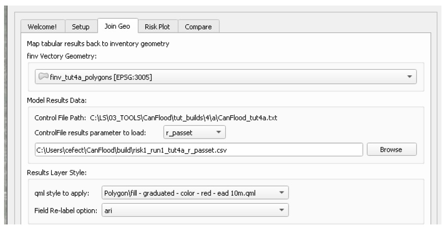
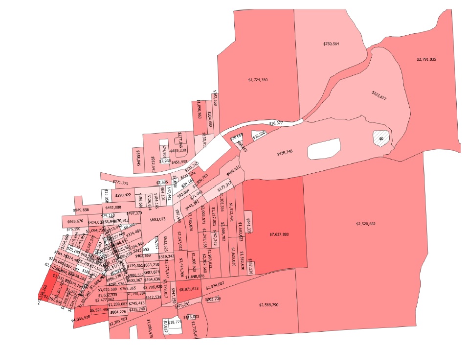
Click ‘Join’. You should see a new polygon vector layer loaded in your canvas with a red graduated style and labels applied to the EAD results calculated in the previous step:
6.9. Tutorial 4b: Risk (L1) with Percent Inundation (Lines)
Like Tutorial 4a, this tutorial demonstrates a risk analysis where the impact metric is percent inundated, but with line geometries rather than polygons. This can be useful for the analysis of flood risk to linear assets like roads.
Load the same data layers from the ‘tutorials4data’ folder, with the addition of:
finv_tut4b_lines.gpkg
Follow all the steps described in Tutorial 4a, but with this new asset inventory (‘finv’) layer.
The per-asset results should look like this:
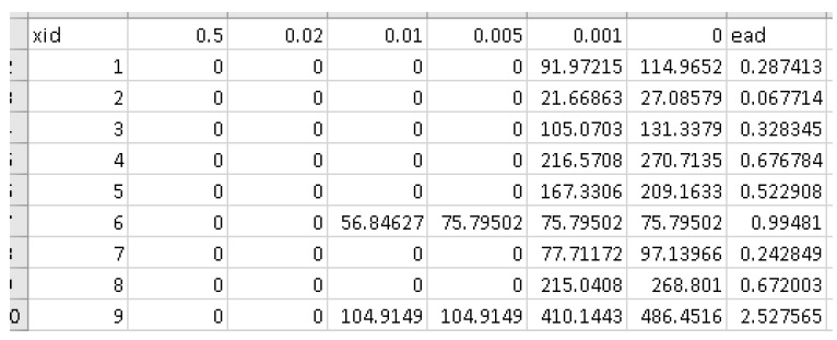
The first non-index ‘impact’ columns represent hazard events, with values showing the percent inundation of each segment multiplied by its ‘f0_scale’ value. This could represent the meters inundated (above the 0.5m depth threshold) per segment, if the ‘f0_scale’ value is the segment length (as is the case with the tutorial inventory). Alternatively, the ‘f0_scale’ value could be set to ‘1.0’ for all features which would cause the values to simply reflect the % inundation of each segment (mirrors the output of the Hazard Sampler tool) and the last column would calculate the expected percent annual inundation of the segment.
6.10. Tutorial 5a: Risk (L1) from NPRI and GAR15
This tutorial demonstrates how to construct a CanFlood ‘Risk (L1)’ model from two web-sources:
The GAR15 Atlas global flood hazard assessment (See Rudari and Silvestro (2015) for details on the GAR15 flood hazard model)
For more information on these data sets, see Appendix A.
Because this tutorial deals with data having disparate CRSs, users should be familiar with QGIS’s native handling of project and layer CRS discussed here.
6.10.1. Load Data to Project
Begin by setting your QGIS project’s CRS to ‘EPSG:3978’ (Project > Properties > CRS > select ‘EPSG:3978’) (Depending on your profile settings, the project’s CRS may be automatically set by the first loaded layer). Now you are ready to download, then add, the data layer for Tutorial 5:
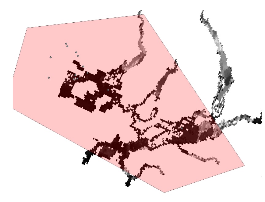
tut5_aoi_3978.gpkg: AOI polygon for tutorial.
Set the AOI’s layer style to ‘fill red transparent’ to allow you to see through the polygon. Before inventory construction can begin, we must add the NPRI and GAR15 raw data to the QGIS project. While there are many options for accessing and importing such data, this tutorial will demonstrate how to use CanFlood’s built-in ‘Add Connections’  feature (Section5.4.1) to first add a connection to the profile, then download the desired layers.
Connect to Web-Data
Begin by expanding the QGIS ‘Browser Panel’ (Ctrl + 2) then clicking ‘Refresh’ on the panel. It should similar to this:
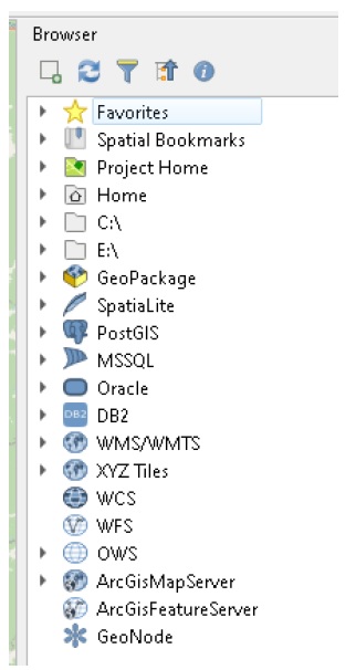
This shows all the connections in your QGIS profile.
Next, execute ‘Add Connections’ (Plugins > CanFlood) to run a script that will attempt to add a set of additional connections to your profile. Your Log Messages should look like this:
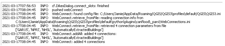
This describes each of the connections that CanFlood added to your profile. To verify this, navigate back to the ‘Browser Panel’. You should see the following connections (under each connection type):
UNISDR_GAR15_GlobalRiskAssessment (WCS)
ECCC_NationalPollutantReleaseInventory_NPRI (ArcGIS Feature Service)
Note that these connections will remain in your profile for future QGIS sessions, meaning the ‘Add Connections’ tool should only be required once per profile (New installations of Qgis should automatically path to the same profile directory (Settings > User Profiles > Open Active Profile Folder), therefore carrying forward your previous connection info).
Download NPRI Data
Now that the connections have been added to your profile, you are ready to download the layers. To limit the data request, ensure your map canvas roughly matches the extents of the AOI (Ctrl+Shift+F will zoom to the project extents). Now open the QGIS ‘Data Source Manager’ (Ctrl + L) and select ‘ArcGIS Feature Server’. Select ‘ECCC_NationalPollutantReleaseInventory_NPRI’ from the dropdown under ‘Server Connections’. Click ‘Connect’ to display the layers available on the server. Select layer 3 ‘Reported releases to surface water for 2019’, check ‘Only request features…’, then click ‘Add’ to add the layer to the project as shown in the following:
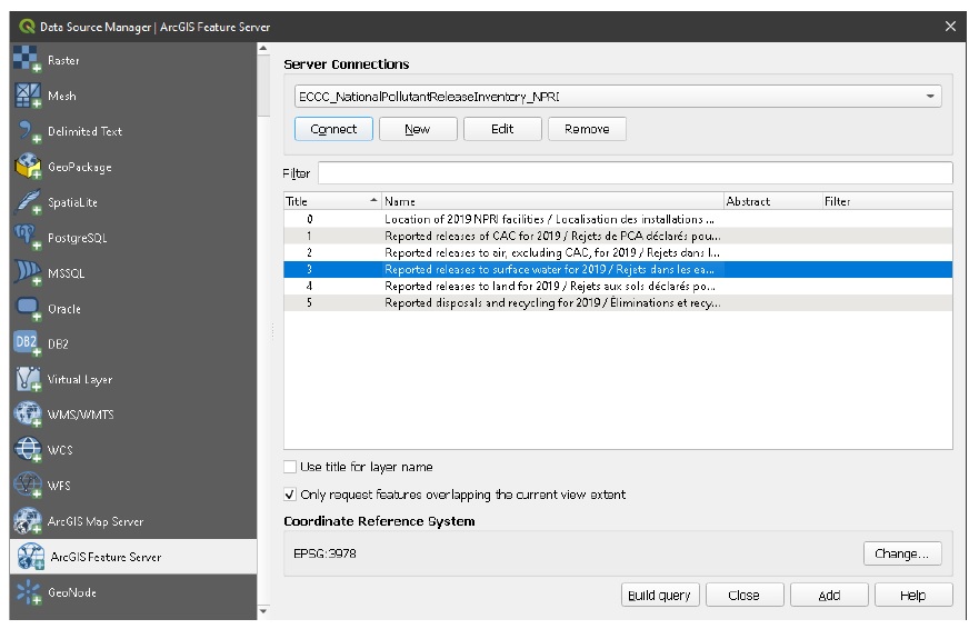
You should now see a vector points layer added to your project with information on each facility reported to the NPRI (within your canvas view). Take note this layer’s CRS is EPSG:3978 (right click the layer in the ‘Layers’ panel > Properties > Information > CRS), this should match your QGIS project and the AOI.
Download GAR15 Data
Follow a similar process to download (Depending on your internet connection, this process can be slow. It’s recommended to set ‘Cache’=’Prefer cache’ to limit additional data transfers, and to turn the layers off or disable rendering once loaded into the project) the following layers from ‘UNISDR_GAR15_GlobalRiskAssessment’ under the ‘WCS’ tab as shown below:
GAR2015:flood_hazard_200_yrp
GAR2015:flood_hazard_100_yrp
GAR2015:flood_hazard_25_yrp
GAR2015:flood_hazard_500_yrp
GAR2015:flood_hazard_1000_yrp
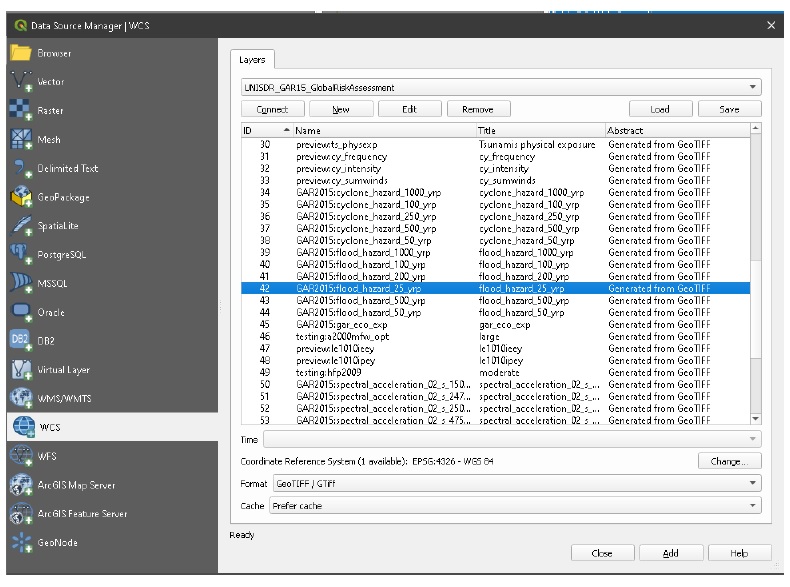
You’ll have to load one layer at a time, and you may be prompted to ‘Select Transformation’ (You can safely select any transformation or close the dialog. These transformations are only for display, we’ll deal with transforming the data onto our CRS below). Once finished, your canvas should look like this:
6.10.2. Build the Model
This section describes how to complete the construction of a Risk (L1) model from the downloaded NPRI and GAR15 data. For instructions on the remainder of the Risk (L1) modelling process, see Section6.1.
Setup
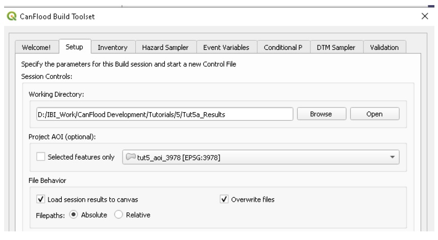
Follow the instructions in Section6.1.2 Setup; however, ensure ‘tut5_aoi_3978’ is selected under ‘Project AOI’ and ‘Load session results…’ is selected.
Construct and Store Inventory
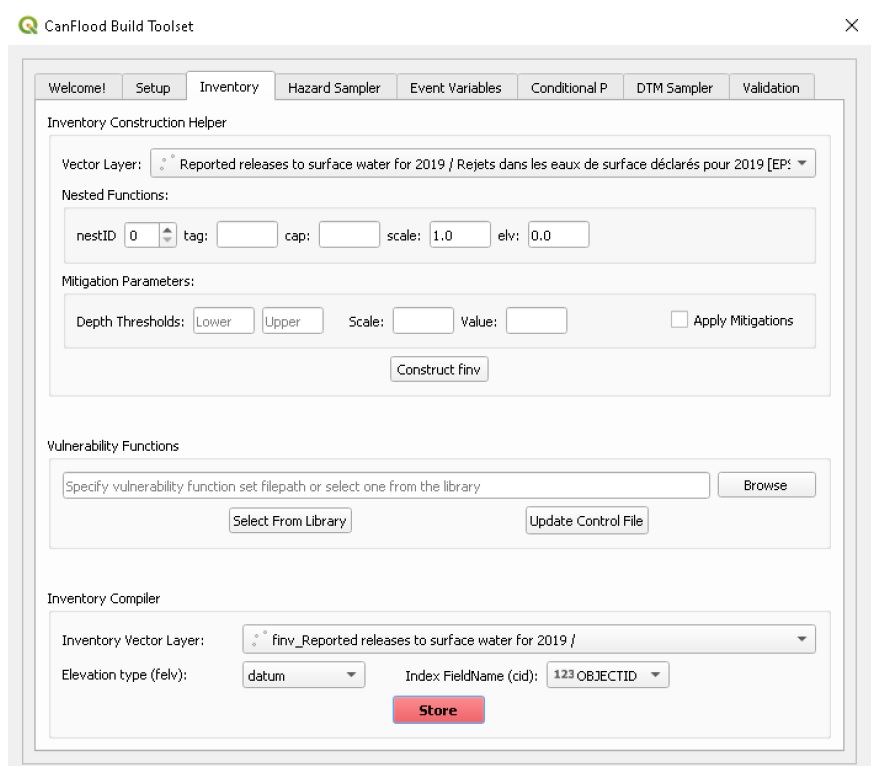
Navigate to the ‘Inventory’ tab. To convert the downloaded NPRI data into an L1 inventory layer that CanFlood will recognize, we need to add ‘elv’ and ‘scale’ fields and values. For this simple analysis, we assume each asset has a vulnerability height of zero (i.e., any positive flood depth leads to exposure). This assumption is accomplished in CanFlood by setting ‘felv’= ‘datum’ and setting each ‘f0_elv’=0 (and using depth rather than WSL rasters). Using the Vector Layer drop down, select the NPRI layer and ensure the ‘nestID’, ‘scale’, and ‘elv’ fields match what is shown below. Finally, click ‘Construct finv’ to build the new inventory layer. To generate the asset inventory (‘finv’) csv file, ensure this new layer is selected in the ‘Inventory Vector Layer’ drop down. Now configure the ‘felv’ and ‘cid’ parameters as shown below, then click ‘Store’:
Hazard Sampler
Now you’re ready to sample the GAR15 hazard layers with your new NPRI inventory. Unlike the hazard layers used in previous tutorials, the GAR15 hazard layers provide depth (rather than WSL) data in centimeters (rather than meters) in a coordinate system other than that of our project. Further, these hazard layers’ extents are much larger than what is needed by our project; and because they are web-layers, many of the QGIS processing tools will not work. Therefore, we’ll need to apply the four ‘Raster Preparation’ tools described in Table5-2 before proceeding with the ‘Hazard Sampler’.
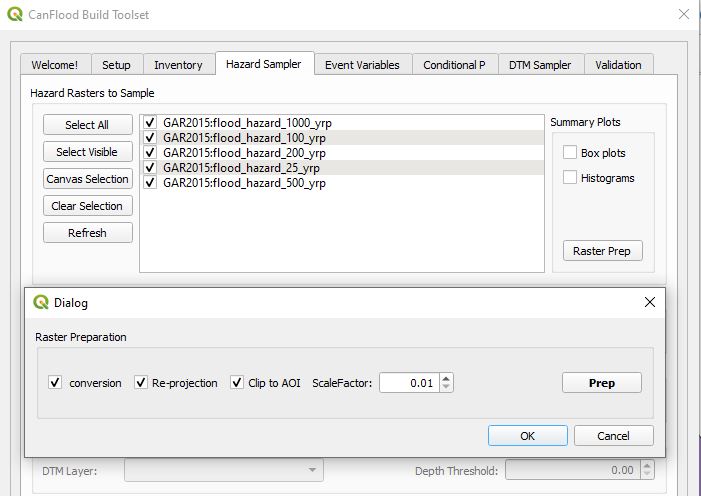
Navigate to the ‘Hazard Sampler’ tab, ensure the five GAR2015 layers are listed in the window, and click ‘Sample’. You should get an error telling you the layer CRS does not match that of the project. To resolve this, click the “Raster Prep’ button and configure the Raster Preparation handles as shown and click ‘Prep’ and then ‘OK’:
You should see five new rasters loaded to your canvas (with a ‘prepd’ suffix). These layers should have rotated pixels, be clipped to the AOI, have reasonable flood depth values (in meters), and have the same CRS as the project (In some cases, QGIS may fail to recognize the CRS assigned to these new rasters, indicated by a “?” shown to the right of the layer in the layers panel. In these cases, you will need to define the projection by going to the layer’s ‘Properties’ and under ‘Source’ set the coordinate system to match that of the project (EPSG: 3978)). Further, each of these rasters should be saved to your working directory. This new set of hazard layers should conform to the expectations of the Hazard Sampler, allowing you to proceed with construction of an L1 model as described in Section6.1.
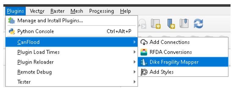
6.11. Tutorial 6a: Dike Failure Polygons
This tutorial demonstrates how to generate ‘failure polygons’ from typical dike information using CanFlood’s ‘Dike Fragility Mapper’ tool (Section5.4.1). Before following this tutorial, users should be familiar with the hazard event data types described in Section4.2 (esp. ‘failure polygons’) that are required of Risk (L1) and (L2) models with some failure. Begin by downloading the tutorial data from the tutorials6 folder and loading it into a new QGIS project:
hazard WSL event rasters (without failure)
o 0010_noFail.tif
o 0050_noFail.tif
o 0200_noFail.tif
o 1000_noFail.tif
dike_influence_zones.gpkg: Dike segment influence area layer with two polygon features, each corresponding to the area of influence of some dike segments;
dikes.gpkg: Dike alignment polyline layer
dtm.tif: Digital Terrain Model (import ‘dtm.qlr’ to get the styled version);
dike_fragility_20210201.xls: Dike fragility function library.
See Section4.5 for a description of these datasets. Ensure your project CRS is set to ‘EPSG:3005’. Once the GIS layers are loaded, your map canvas should look similar to the below:
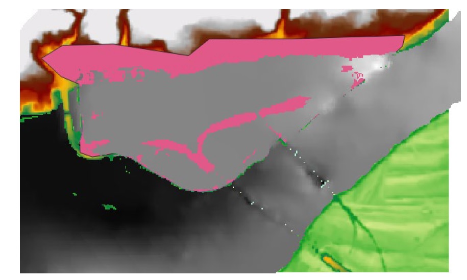
To make this workspace more friendly, ensure the ‘dikes’ and ‘dike_influence_zones’ layers are at the top of the layers panel. Now apply the following CanFlood styles (Load these styles onto your profile using the Plugins>CanFlood>Add Styles tool described in Section5.4.4) to each of these layers:
dikes: ‘arrow black’
dike_influence_zones: ‘fill red transparent’
The arrow style is useful as we’ll need to know the directionality of the dike layer to tell the tool which side of the dike to sample. Now we’re ready to open the ‘Dike Fragility Mapper’ dialog:
Configure your dialog similar to what is shown below but using your own directories (ensure ‘dikeID’ is set to ‘ID’):
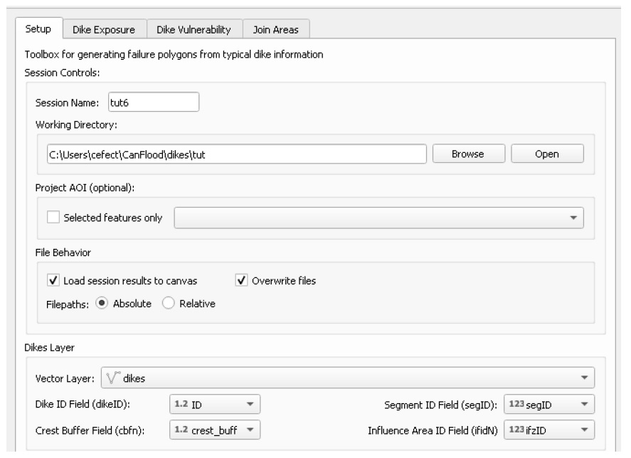
6.11.1. Calculate Dike Exposure
This step will calculate the exposure, or freeboard, values of each dike segment. Navigate to the ‘Dike Exposure’ tab, click ‘Refresh’, then configure it as shown below, taking care to select the DTM layer in the drop-down, but not in the selection window:
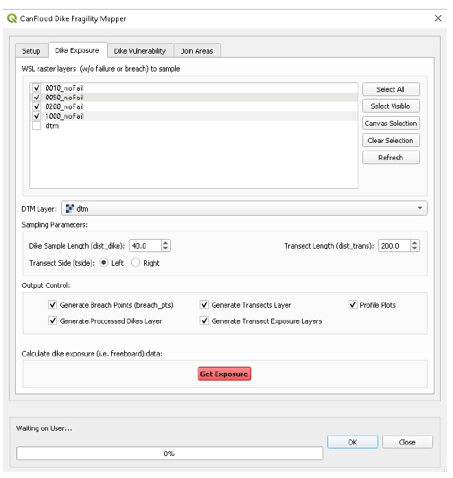
Click ‘Get Exposure’. You should see 10 layers loaded under the ‘CanFlood.Dikes’ group:
tut6_dike_dikes: processed dikes layer
breach points layers (for each event)
o 0010_noFail_breach_1_pts
o 0050_noFail_breach_3_pts
o 0200_noFail_breach_16_pts (see below
)
o 1000_noFail_breach_50_pts
tut6_tut6_dike_dikes_transects: transects layer (see below
)
transect exposure points layers
o tut6_dike_dikes_0010_noFail_expo
o tut6_dike_dikes_0050_noFail_expo
o tut6_dike_dikes_0200_noFail_expo (see below
)
o tut6_dike_dikes_1000_noFail_expo
These layer types are explained in Section6.11, and those relevant to the 200-year series are displayed below. The 40 m dike sample length and 200 m transect length we specified in the dialog box can be seen in the spacing and length of the transects shown below:
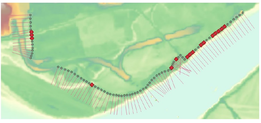
At its core, this tool samples the WSL raster at the tail of each transect and the DTM at the head, then compares these to calculate the freeboard. This suggests the user must specify an appropriate transect side, sample length, and transect length based on the configuration of diking and flooding to obtain an accurate freeboard calculation.
To visualize the calculated freeboard values, apply ‘Single Labels’ for the ‘sid’ values on the processed dikes layer, then navigate to your working directory and open the ‘tut6 dike 43-1 profiles.svg’ image file. It should look similar to the below:
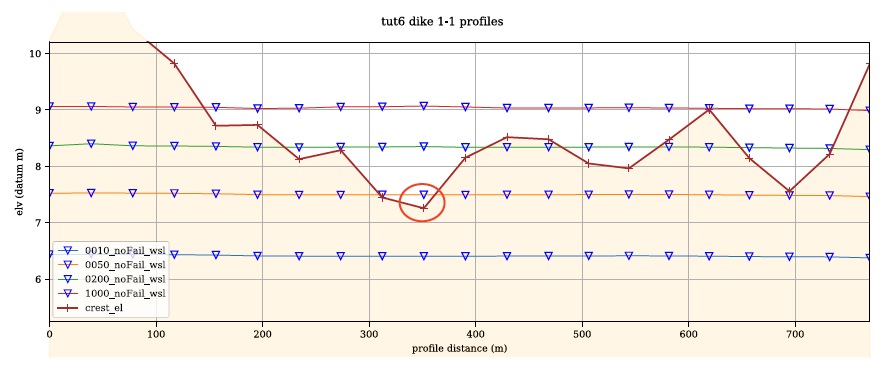
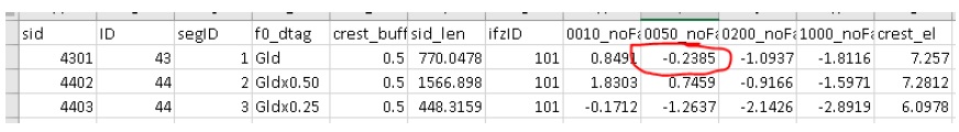
This is a profile plot of dike 43, segment 1 (sid=4301) showing the calculated crest elevation and WSL for the four event rasters (sampled with each transect). Note that, this plot suggests the freeboard of the 50-year to be around -0.2 m (see red circle above). Now open the ‘tut6_dExpo_7_3.csv’ file in the working directory, this is the dike segment exposure (‘dexpo’) dataset that we’ll use in the next step to calculate failure probabilities. Notice the freeboard value of the segment-event in question is -0.2m as expected:
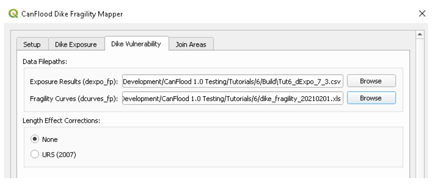
6.11.2. Calculate Dike Vulnerability
This step will use the previously calculated freeboard values and the user supplied fragility curves to calculate the probability of failure of each segment. Switch to the ‘Dike Vulnerability’ tab, you should see the filepath to the above exposure results automatically populated in the ‘dexpo_fp’ field. Now select the fragility curves library ‘dike_fragility_20210201.xls’ file provided with the tutorial data. The tab-names in this workbook correspond to ‘f0_dtag’ field on the dikes layer, telling CanFlood which curve to apply to which segment. Choose ‘None’ for the length effect corrections. Your dialog should look similar to this:
Now click ‘Calc Fragility’ to generate the tabular failure probability data (‘pfail’).
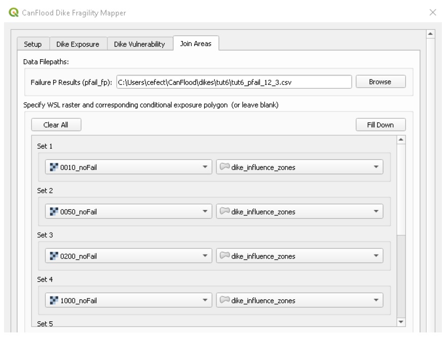
6.11.3. Join to Areas
In this final step, we will join the previously calculated failure probabilities to the user supplied influence areas for each segment based on the links provided on the dikes layer. Navigate to the ‘Join Areas’ tab. You should see the ‘pfail’ data filepath in the corresponding field; if not, navigate to this file. If you successfully ran the ‘Dike Exposure’ tool this session, you should see the first column of raster layers selected; if not, select the four WSL rasters manually in the first column. For the second column, select the ‘dike_influence_zone’ polygon layer in the first drop-down, then click ‘Fill Down’ to populate the remaining drop-downs. Once finished, your dialog should look like the below:
Click ‘Map pFail’. You should see four polygon layers loaded to your canvas, one for each event. Move these layers up on the layers list so they display on top of the rasters. The 200-year is shown below:
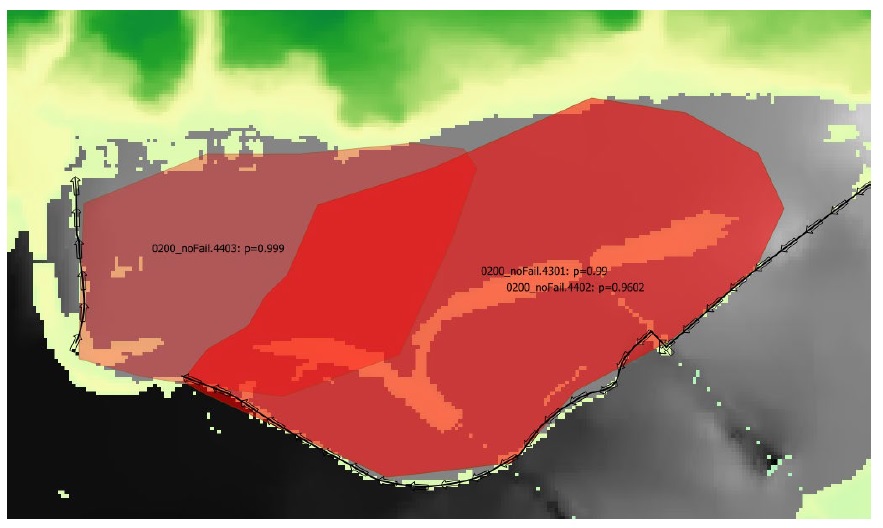
These results layers are automatically stylized as failure polygons, showing the event raster name, source dike segment (‘sid’), and failure probability of each feature. Notice the 200-year contains 3-overlapping polygon features corresponding to the three segments with failure here, despite the original ‘dike_influznce_zones’ layer having two features. This mapping of polygons to dike segments is set on the dikes layer in the ‘Influence Area ID Field’ specified on the ‘Setup’ tab (‘ifzID’ in this case). In this way, 1:1 or many:many segment-polygon links can be specified, allowing the user to map each breach probability, or group segments to apply the calculated probabilities to a larger dike ring. See Section5.4.1 for more information on this tool.
6.12. Tutorial 7a: Sampling on Complex Geometries
This tutorial demonstrates Value Sampling using sampling statistics specified Per-Asset. This can be useful when you would like to sample using heterogeneous statistics within a single inventory (e.g., ‘Max’ ground elevation for some buildings and ‘Min’ elevation for others). Begin by downloading the tutorial data from the tutorials 7 folder and loading it into a new QGIS project:
haz_rast: hazard event rasters with WSL value predictions for the study area for four probabilities.
o haz_0050_tut4.tif
o haz_0100_tut4.tif
o haz_0200_tut4.tif
o haz_1000_tut4.tif
dtm_cT2.tif: DTM layer (and corresponding stylized layer definition .qlr file)
finv_tut7_polys.gpkg: flood asset inventory (’finv’) spatial layer (and corresponding stylized layer definition .qlr file)
6.12.1. Build the Model
Setup
Complete the typical setup as instructed in Tutorial 1a.
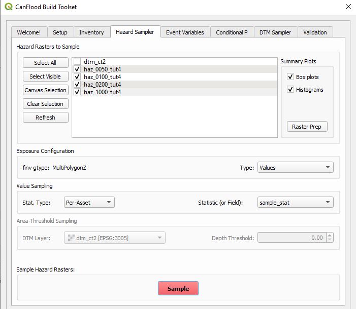
Hazard Sampler
Navigate to the ‘Hazard Sampler’ tool, check mark the four hazard rasters, set the ‘Type’ parameter to ‘Values’, set the ‘Stat. Type’ parameter to ‘Per-Asset’, then select the ‘sample_stat’ field to tell CanFlood to pull the sampling statistic from this field. Verify your dialog looks like the below then click ‘Sample’.
Complete the rest of the build process by running the ‘Event Variables’, ‘DTM Sampler’ and ‘Validation’ tools as outlined in Tutorial 1a.
6.12.2. Run the Model
Open the ‘Model’ dialog and follow the steps in Tutorial 1a to setup this model run. Then execute the ‘Risk (L1)’ model to generate the following files:
risk1_tut7a_passet.csv: expected value of inundation per asset;
risk1_tut7a_ttl.csv: total results, expected value of total inundation per event;
tut7a.run1 Impact-ARI plot on 6 events.svg: a plot of the total results.
In order to understand and visualize the effect of setting the hazard sampling statistic to ‘Per-Asset’, you can try re-building and running the same model with the hazard statistic type set to ‘Global’ and the statistic set to ‘Mean’, then compare the results.
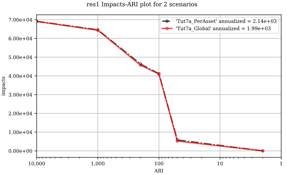
6.12.3. View Results
To visualize the difference between these two model configurations, open the ‘Results’ toolset and select a working directory and the original ‘Per-Asset’ control file as the ‘main control file’ on the ‘Setup’ tab. Before generating the comparison files, configure the plot style by opening the same main control file, and changing the following ‘[plotting]’ parameters:
‘color = red’
‘linestyle = solid’
‘impactfmt_str = ,.0f’
To generate a comparison plot of these two scenarios, navigate to the ‘Compare/Combine’ tab, select the ‘Control File’ for both model configurations (Per-Asset & Global) generated in the previous step, ensure ‘Control Files’ is checked under ‘Comparison Controls’ then click ‘Compare’. Your results should look similar to this:
6.13. Tutorial 8a: Sensitivity Analysis
This tutorial demonstrates Sensitivity Analysis workflow (Section5.4.5). This can be useful for quantifying the sensitivity of your model to each parameter and datafile.
Begin by downloading the tutorial data from the tutorials 8 folder and loading it into a new QGIS project:
haz_rast: hazard event rasters with WSL value predictions for the study area for four probabilities.
o haz_0050_tut8.tif
o haz_0100_tut8.tif
o haz_0200_tut8.tif
o haz_1000_tut8.tif
dtm_tut8.tif: DTM layer (and corresponding stylized layer definition .qlr file)
finv_tut8.gpkg: flood asset inventory (’finv’) spatial layer (and corresponding stylized layer definition .qlr file)
CanFlood_tut8.txt: main model control file
6.13.1. Setup the Analysis
Launch the Sensitivity Analysis  dialog from the Plugins>CanFlood menu. Navigate to the Setup menu, select your working directory, set the filepaths to ‘relative’, then specify your main model control file and ‘Model Level’ = ‘L2’ as shown below:
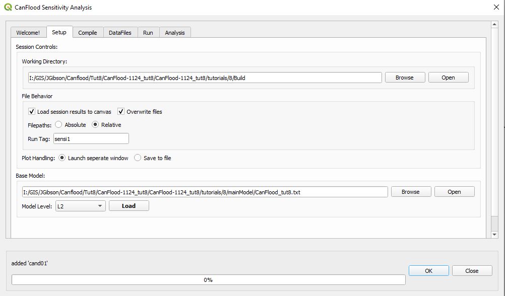
Click Load to populate the Compile tab.
6.13.2. Configure and Compile the Model Suite
Navigate to the Compile tab. It should have been automatically populated with the ‘base’ values from the control file on the first row, and a duplicate of this on the second row:
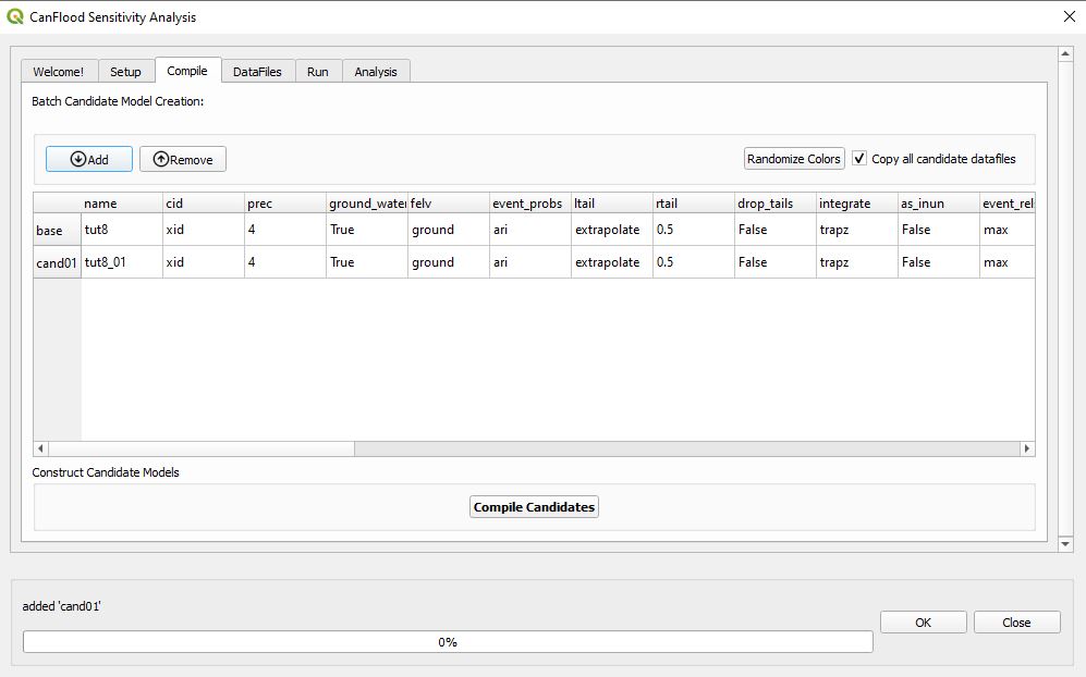
Now add three more candidate models by clicking the ‘Add’ button three times. Notice the model names have been automatically generated, but the remaining fields are identical to the base model. Now we’ll modify or ‘perturb’ one parameter or datafile on each candidate to compile the sensitivity analysis suite.
For the first perturbation, simply change the rtail value on ‘cand01’ to 0.1. For the second perturbation, change the ‘curve_deviation’ on ‘cand02’ to ‘lo’ to match the lower bound depth-damage values stored in the curves.xls. We will configure the remaining two perturbations in the following step.
To allow us to differentiate the plots we generate (see below), click ‘Randomize Colors’.
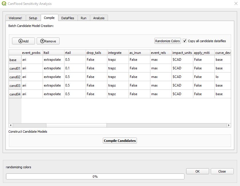
Ensure ‘Copy all candidate data files’ is selected so the compiler will give each candidate its own data files, rather than have each point back to the main model’s datafiles. Finally, click ‘Compile Candidates’. You will now see four new folders, one for each candidate model, in your working directory.
6.13.3. Manipulate Datafiles
On the DataFiles tab, select ‘cand03’ and ‘finv’ to populate the datafile path with the corresponding datafile. Click ‘Load’ to add this datafile as a memory layer to your project.
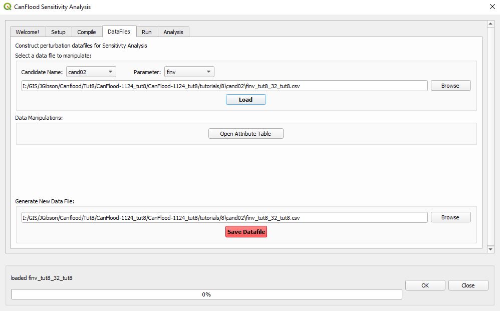
Now we’ll subtract 0.5 m from f0_elvs. click ‘Open Attribute Table’ (or the corresponding button on the QGIS toolbar, or hit ‘F6’) to open the attribute table window. Make a mental note of the ‘f0_elv’ values. Now open the Field Calculator (Ctrl + I). Check ‘Update Existing Field’ and select ‘f0_elv’ from the combobox. Select the custom ‘finv_elv_add’ expression function from the ‘CanFlood’ menu in the middle and complete the expression ass shown:
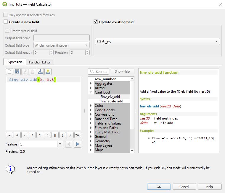
Click ‘OK’ to make the change to the field values. Examine the ‘f0_elv’ values in the attribute table, they should now be 0.5 less than before (i.e., 0.5 less than the base model).
Back on the ‘DataFiles’ tab, click ‘Save Datafile’ to overwrite the old csv with your modifications.
For our final perturbation, we’ll subtract 0.5 m from the ground elevations (‘gels’). Select ‘cand04’ and ‘gels’ then click ‘Load’ to load this datafile. Follow a similar procedure as above to setup the Field Calculator and enter the formula shown below:
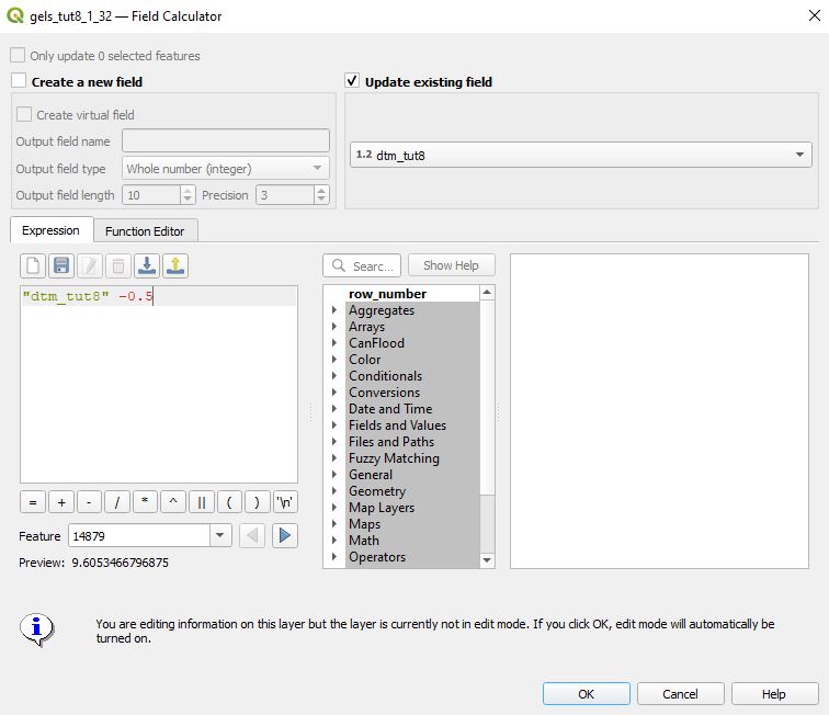
Click ‘OK’ on the Field Calculator to update the values. click ‘Save Datafile’ to write these changes to the csv.
6.13.4. Run the Suite
On the Run tab you should see the base model and the four new candidate model control files shown:
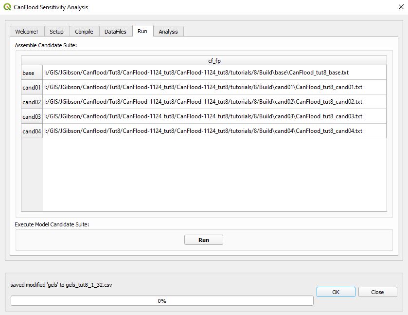
Click Run to bulk run these L2 CanFlood models.
6.13.5. Analyze the Results
On the Analysis tab, you should see the run suite results .pickle file loaded, the summary values, and the summary table populated:
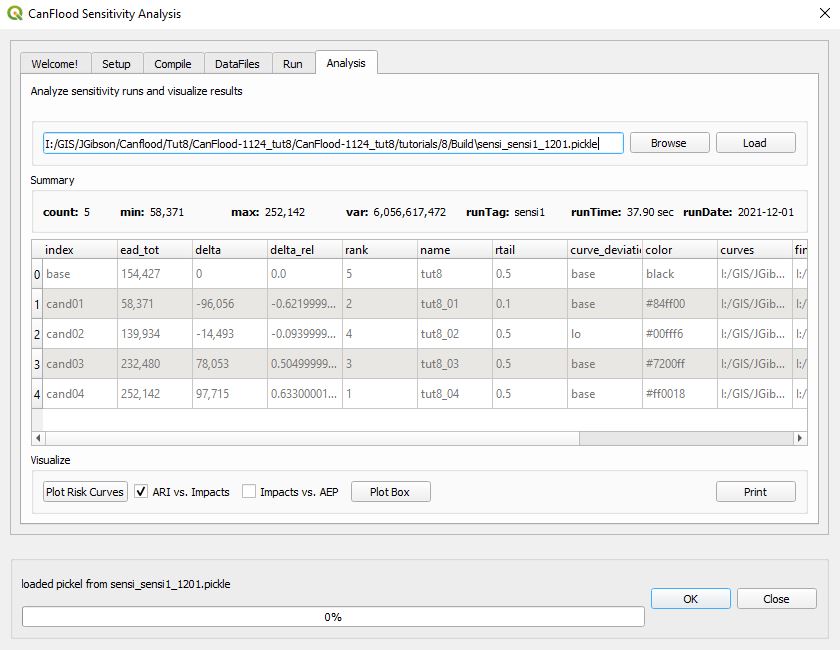
Click ‘Plot Risk Curves’ to obtain the comparison risk curves for this suite:

From this plot, you can clearly see the influence of the ‘rtail’ parameter on the risk curve (and the annualized metric). The lowering of the ground elevations and the main floor elevations produced expectedly similar results.