5. Toolsets

This section describes the use and function of CanFlood’s toolsets in detail.

5.1. Build

The build toolset contains a suite of tools summarized in Table5-1 intended to aid the flood risk modeller in their construction of CanFlood L1 and L2 models.

Table 5-1: Build tools summary

Tab Name	Tool Name	Description	Inputs	Outputs
Setup	Start Control File	Creates a Control File template	name and precision	Control File Template
Inventory	Inventory Constructor	Builds a finv template	vector layer, attributes	inventory vector layer (‘finv’)
Inventory	Vuln. Function Library	GUI for selecting a Function set		Vulnerability Function Set
Inventory	Inventory Compiler	Clip and extract finv data to tabular format	‘finv’, parameters	inventory tabular data (‘finv’)
Hazard Sampler	Raster Preparation	Manipulate hazard rasters	hazard rasters	hazard rasters
Hazard Sampler	Sample Rasters	Sample hazard raster values	hazard rasters, ‘finv’, DTM	exposure dataset (‘expos’)
Event Variables	Store Evals	Write event probabilities to file	hazard event probabilities	event variables (‘evals’)
Conditional P	Conditional P	Resolve conditional exposure probabilities	‘finv’, failure polygons	exposure prob.(‘exlikes’)
DTM Sampler	DTM Sampler	Sample DTM raster at asset geometry	‘finv’, DTM	ground elevations (‘gels’)
Validation	Validation	Validate against model requirements	complete model package

5.1.1. Setup

This tab facilitates the creation of a Control File from user specified parameters and inventory, as well as providing general file control variables for the other tools in the toolset.

5.1.2. Inventory

The inventory tab contains a set of tools for constructing and converting flood asset inventories (‘finv’; Section4.1). The remainder of this section describes the available inventory tools.

Inventory Construction Helper

The optional ‘Inventory Construction Helper’ tool helps construct a Flood Asset Inventory template from some vector geometry within CanFlood’s ‘nested function’ framework (Section4.1). Additional data analysis outside the CanFlood platform is generally required to populate these fields.

Vulnerability Function Library

To support the construction of preliminary risk models, the CanFlood plugin provides a collection of vulnerability function libraries commonly used in Canada. Users should carefully study legacy vulnerability functions and their construction methods before incorporating them into any risk analysis. At a minimum, functions should be scaled to account for spatial and temporal transfers.

Inventory Compiler

The Inventory Compiler is a simple tool used to prepare an inventory vector layer for inclusion in a CanFlood model using the following process:

1. clip the selected vector layer by the AOI (if one is selected on the Setup tab);

2. extract non-spatial data to the working directory as a csv; and

3. write the file location of this csv and the Index FieldName to the control file.

5.1.3. Hazard Sampler

The Hazard Sampler tool generates the exposure dataset (‘expos’) from a set of hazard event rasters. Generally, these hazard event rasters represent the WSL results of some hazard model (e.g. HEC-RAS) at specific probabilities. The hazard sampler has two basic modes:

• Value Sampling: Sample raster values at each asset; generally the default when you’re interested in the depth at an asset. For line and polygon assets, this requires the user specify a sampling statistic (either globally or per-asset).

• Area-Threshold Sampling: Calculate the percent-of each asset length or area above some threshold raster value; useful for calculating the percent of inundation of road segments or agricultural crop polygons. This requires a DTM layer and a ‘Depth Threshold’ be specified.

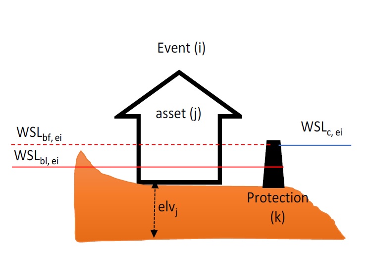
Figure 5-1: Risk calculation definition diagram where the dashed line is the WSL value of event ‘ei’

Using the definitions in Figure5-1, the WSL exposure from an event i to a single asset j with height elv _j is calculated as:

expo _i,j = WSL _{bl, ei} - elv _j

The hazard sampler performs the following general steps to the set of user-supplied hazard layers and inventory layer:

1. Slice the inventory layer by the AOI (if ‘Project AOI’ is specified)

2. For each layer, sample the raster value or calculate the percent inundation of each asset;

3. Save the results in the ‘expos’ csv file to the working directory and write this path to the Control File;

4. Load the results layer to canvas (optional)

Value Sampling for Complex Geometries

Unlike Point geometries, inventories with line or polygon geometries require some sampling statistic (e.g., ‘Min’, ‘Max’, ‘Mean’) to tell CanFlood how the raster value should be calculated from each asset geometry. Two options for specifying the sampling statistic are provided:

• Global: A single sampling statistic is specified and used for all asset geometries (e.g., take the ‘Max’ raster value encountered within each polygon).

• Per-Asset: A sampling statistic is specified for each asset via some field value on the inventory (e.g., take the ‘Max’ value for some assets and the ‘Min’ value for others). This is most useful for large asset geometries and rasters with high variance (e.g., building polygons sampling DTMs in areas with significant terrain)

Raster Preparation

The raster sampler expects all the hazard layers to have the following properties:

• layer CRS matches project CRS;

• layer pixel values match those of the vulnerability functions (e.g., values are typically meters);

• layer dataProvider is ‘gdal’ (i.e., the tool does not support processing web-layers).

To help rasters conform to these expectations, CanFlood includes a ‘Raster Preparation’ feature on the ‘Hazard Sampler’ tab with the tools summarized in Table5-2.

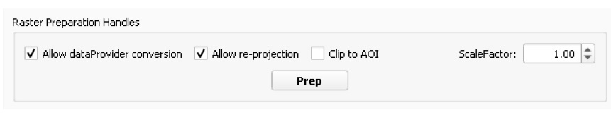
Table 5-2: Raster Preparation tools

Tool Name	Handle	Description
Downloader	Allow dataProvider conversion	If the layer’s dataProvider is not ‘gdal’ (i.e., web-layers), a local copy of the layer is made to the user’s ‘TEMP’ directory.
Re-projector	Allow re-projection	If the layer’s CRS does not match that of the project, the ‘gdalwarp’ utility is used to re-project the layer.
AOI clipper	Clip to AOI	This uses the ‘gdalwarp’ utility to clip the raster by the AOI mask layer.
Value Scaler	ScaleFactor	For ScaleFactors not equal to 1.0, this uses the Raster Calculator to scale the raster values by the passed ScaleFactor (useful for simple unit conversions).

After executing these tools, a new set of rasters are loaded to the project.

Sampling Geometry and Exposure Type

To support a wide range of vulnerability analysis, the Hazard Sampler tool is capable of developing WSL and inundation exposure variables from the three basic geometry types as shown in Table5-3. For line and polygon type geometries, the tool requires the user to specify the sample statistic for WSL calculations, and a depth threshold for percent inundation calculations.

Table 5-3: Hazard Sampler configuration by geometry type and exposure type and [relevant tutorial.]

Geometry	WSL			Inundation
	Parameters	Exposure		Parameters		Exposure
Point	Default [Tutorial 2a]	WSL		Default [Tutorial 1a]		WSL 1
Line 4	Sample Statistic 3, 5	WSL Statistic		% inundation, Depth Thresh 2 [Tutorial 4b]		% inundation
Polygon 4	Sample Statistic 3	WSL Statistic		% inundation, Depth Thresh 2 [Tutorial 4a]		% inundation
To apply a threshold depth, the f_elv values can be manually manipulated. WSL exposure values are converted to binary-exposure (i.e., inundated or not inundated) by the Risk (L1) model. Requires a DTM raster be specified on the ‘DTM Sampler’ tab. Model tools expect the asset inventory (‘finv’) to contain a ‘f_elv’ column with all zero values and parameter.felv=’datum’. Respects NULL raster cell values as not inundated. Ignores NoData values when calculating statistics. M and Z values are not supported. Throws a ‘feature(s) from input layer could not be matched’ error when null values are encountered. This error is safe to ignore.

5.1.4. Event Variables

The Event Variables ‘Store Evals’ tool stores the user specified event probabilities into the event variables (‘evals’) dataset. The Hazard Sampler tool must be run first to populate the Event Variables table.

Notes and Limitations

The following apply to the Event Variables and connected tools:

• The Risk (L1 and L2) modules require at least 3 events unique event probabilities.

5.1.5. Conditional P

To incorporate defense failure (Section1.4), CanFlood ‘Risk (L1)’ and ‘Risk (L2)’ models expect a resolved exposure probabilities (‘exlikes’) data set that specifies the conditional exposure probability of each asset to each hazard failure raster. The ‘Conditional P’ tool provides a conversion from a collection of failure influence area polygons and rasters (i.e., the outputs of a flood protection reliability analysis) to the resolved exposure probabilities (‘exlikes’) dataset. For each conditional failure event, the ‘Conditional P’ tool expects the user to provide a pair composed of the following layers:

• Raster of WSL that would be realized in the failure event

• Vector layer with polygon features indicating the extent and probability of element failures during the hazard event (‘failure polygons’). These features can be non-overlapping (simple conditionals) or overlapping (complex conditionals) as discussed below.

The user can specify up to eight event-raster/conditional-exposure-probability-polygon pairings with the GUI.

CanFlood distinguishes ‘complex’ and ‘simple’ conditional exposure probability polygons based on the geometry overlap of their features as summarized in Table5-4 and shown in Figure5-2.

Table 5-4: Conditional exposure probability polygon treatment summary.

Type	Features	Treatment	Example (Figure 5-5)
trivial	none	Failure not considered, no resolved exposure probabilities (‘exlikes’) required	n/a
simple	not overlapping	‘Conditional P’ tool joins the specified attribute value from the polygon feature onto each asset to generate resolved exposure probabilities (‘exlikes’).	f2, f3
complex	overlapping	see below	f1

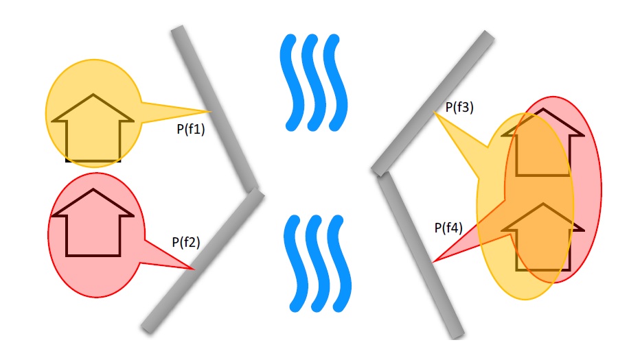
Figure 5-2:Simple [left] vs. Complex [right] conditional exposure probability polygon conceptual diagram showing a single layer with four features.

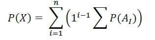
For complex conditionals, ‘Conditional P’ provides two algorithms to resolve overlapping failure polygons down to a single failure probability (for a given asset on a given failure raster) based on two alternate assumptions for the mechanistic relation between the failure mechanisms summarized in Table5-5.

Table 5-5: Conditional exposure probability polygon resolution algorithms for complex conditional

Relation	Algorithm Summary
Mutually Exclusive
Independent 1
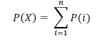
Where P(X) is the resolved failure probability for a single asset on a given event and P(i) isthe failure probably value sampled from a failure polygons feature. Bedford and Cooke (2001)

5.1.6. DTM Sampler

The DTM Sampler tool uses the same module as the Hazard Sampler to sample DTM raster values at each asset provided in the inventory vector layer. This tool outputs the ground elevation (‘gels’) dataset and writes the corresponding reference to the control file. This dataset is required by any model where the inventory (‘finv’) data’s height or elevation parameters are specified relative to ground (felv=’ground’).

5.1.7. Validation

The Validation tool performs a series of checks on the specified control file to ensure the data requirements of the specified model are satisfied. If the checks are satisfied, the corresponding validation flag is set in the control file, allowing the model tool to run.

5.2. Model

The ‘Model’ toolset provides a GUI to facilitate access to CanFlood’s 3 flood risk models. CanFlood’s L2 models are split between exposure and risk to facilitate custom applications (these can be linked using the ‘Run Risk Model (L2)’ checkbox). The following tabs are implemented in CanFlood’s Model toolset:

• Setup: Filepaths, run descriptions, and optional parameters used by all Model tools;

• Risk (L1): Inundation likelihood analysis;

• Impacts (L2): Part one of the L2 models, exposure per event calculated with vulnerability functions;

• Risk (L2): Part two of the L2 models, expected value of all event impacts;

• Risk (L3): SOFDA research model

Batch Runs

To facilitate batch simulations for advanced users, all CanFlood modelling modules have reduced dependency requirements (e.g. the QGIS API is not required).

Parameter Summary

The following table summarizes the relevant parameters for CanFlood’s model toolset that can be specified in the Control File

CanFlood control file parameter summary

name	option	type expectation	default	description
name		str		name of the scenario/model run
cid				index column for the 3 inventoried data sets (finv expos gels)
prec		int		float precision for calculations
ground_water		bool		flag to include negative depths in the analysis
felv		str		datum or ground
event_probs		str	ari	format of event probabilities (in evals data file) .
	aep			event probabilities in aeps file expressed as annual exceedance probabilities
	ari			expressed as annual recurrance intervals
ltail		None	extrapolate	zero probability event handle
	flat			zero probability event equal to the most extreme impacts in the passed series
	extrapolate			set the zero probability event by extrapolating from the most extreme impact (interp1d)
	none			do not extrapolate (not recommended)
	float			use the passed value as the zero probability impact value
rtail		None	0.5	zero impacts event handle
	extrapolate			set the zero impact event by extrapolating from the least extreme impact
	none			no enforcing of a zero impact event (not recommended)
	flat			duplicates the minimum AEP as the zero damage event (NOT IMPLEMENTED)
	float			use the passed value as the zero impacts aep value
drop_tails		bool	FALSE	EAD extrapolation: whether to remove the extrapolated values before writing the per asset results
integrate		str		numpy integration method to apply (default trapz)
as_inun		bool		flag whether to treat exposures as %inundation
event_rels		str		assumption for calculated expected value on complex events
	max			maximum expected value of impacts per asset from the duplicated events resolved damage = max(damage w/o fail damage w/ fail * fail prob) default til 2020-12-30
	mutEx			assume each event is mutually exclusive (only one can happen) (lower bound)
	indep			assume each event is independent (failure of one does not influence the other) (upper bound)
impact_units		str		value to label impacts axis with (generally set by Dmg2)
apply_miti		bool		whether to apply mitigation algorthihims
curve_deviation		str		for L2 damage function libraries, specify the deviation (optional)

CanFlood control file datafile and plotting summary

section	name	type expectation	description
dmg_fps	curves	str	for L2 filepath to damage function library .xls
	finv	str
	expos	str
	gels	str
risk_fps	dmgs	str	damage data results file path (default N/A)
	exlikes	str	secondary exposure likelihood data file path (default N/A)
	evals	str	event probability data file path (default N/A)
validation	risk1	bool
	dmg2	bool
	risk2	bool	Risk2 validation flag (default False)
	risk3	bool
results_fps	attrimat02	str	lvl2 attribution matrix fp (post dmg model)
	attrimat03	str	lvl3 attribution matrix fp (post risk model)
	r_passet	str	per_asset results from the risk2 model
	r_ttl	str	total results from riskModels
	eventypes	str	df of aep noFail and rEventName
plotting	color	str
	linestyle	str
	linewidth	float
	alpha	float
	marker	str
	markersize	float
	fillstyle	str
	impactfmt_str	str	python formatter to use for formatting the impact results values

Some of these can be configured with CanFlood’s Build toolset UI, while others must be specified manually in the Control File.

5.2.1. Risk (L1)

CanFlood’s L1 Risk tool provides a preliminary assessment of flood risk with binary exposure as discussed in Section3.1. This tool also supports conditional probability inputs to incorporate flood protection failures. Table5-6 summarizes the input requirements for the Risk (L1) model, which are generally prepared using the ‘Build’ tools (Figure3-1).

Table 5-6: Risk (L1) CanFlood model package requirements.

Name	Description	Build Tool	Code	Reqd.
Control File	Data file paths and parameters	Start Control File		yes
Inventory	Tabular asset inventory data	Inventory Compiler	finv	yes
Exposure	WSL or %inundated exposure data	Hazard Sampler	expos	yes
Event Probabilities	Probability of each hazard event	Event Variables of applicable	evals	yes
Exposure Probabilities	Conditional probability of each asset realizing the failure raster	Conditional P	exlikes	for failure
Ground Elevations	Elevation of ground at each asset	DTM Sampler	gels	for felv=ground

The Risk (L1) module can be used to estimate a range of simple-metrics through creative use of the asset inventory (‘finv’) fields discussed in Section4.1. When the ‘scale’ factor is set to 1, ‘height’ to zero, and no conditional probabilities are used (typical for inundation analysis), most of the calculation becomes trivial as the result is simply the impact values provided by the ‘expos’ table (with the exception of the expected value calculation).

Outputs provided by this tool are summarized in the following table:

Table 5-7: Risk model output file summary.

Output Name	Code	Description
total results	r_ttl	table of sum of impacts (for all assets) per event and expected value of all events (EAD)
per-asset results	r_passet	table of impacts per asset per event and expected value of all events per asset
risk curve		risk curve plot of total impacts

5.2.2. Impacts (L2)

CanFlood’s Impacts (L2) tool is designed to perform a ‘classic’ object-based deterministic flood damage assessment using vulnerability curves, asset heights, and WSL values to estimate flood impacts from multiple events. This tool calculates the impacts on each asset from each hazard event (if the provided raster WSL was realized). ‘Impacts (L2)’ does not consider or account for event probabilities (conditional or otherwise) as these are handled in the Risk (L2) module (see Section5.2.3). Model package requirements are summarized in the following table:

Table 5-8: Impacts (L2) model package requirements.

Name	Description	Build Tool	Code	Reqd.
Control File	Data file paths and parameters	Start Control File		yes
Inventory	Tabular asset inventory data	Inventory Compiler	finv	yes
Exposure	WSL or %inundated exposure data	Hazard Sampler	expos	yes
Ground Elevations	Elevation of ground at each asset	DTM Sampler	gels	for felv=ground
Vulnerability Function Set	Collection of functions relating exposure to impact	Vulnerability Function Library	curves	yes

Impacts (L2) outputs are summarized in the following table, where only the ‘dmgs’ output is required by the Risk (L2) model:

Table 5-9: Impacts (L2) outputs.

Output Name	Code	Description
total impacts	dmgs	total impacts calculated for each asset
expanded component impacts	dmgs_expnd	complete impacts calculated on each nested function of each asset (see below)
impacts calculation summary	bdmg_smry	workbook summarizing components of the impact calculation (see below)
depths	depths_df	depth values calculated for each asset
impact histogram summary		summary plot of total impact values per-asset
impact box plot		summary plot of total impact values per-asset

Nested Functions

To facilitate complex assets (e.g. a house vulnerable to structural and contents damages), Impacts (L2) supports composite vulnerability functions parameterized with the 4 key attributes (‘tag’, ‘scale’, ‘cap’, ‘elv’) with the ‘f’ prefix and ‘nestID’ numerator (e.g. f0, f1, f2, etc.) discussed in Section4.1. In this way, CanFlood can simulate a complex vulnerability function by combining the set of simple component functions to estimate flood damage. An example entry in the asset inventory (‘finv’) for a single-family dwelling may look like:

xid	f0_tag	f0_scale	f0_cap	f0_elv	f1_cap	f1_elv	f1_scale	f1_tag
14879	BA_S	117.99	91300	11.11	20000	11.11	117.99	BA_C

Where BA_S corresponds to a vulnerability function for estimating structural cleanup/repair, and BA_C estimates household contents damages (both scaled by the floor area). Additional fX columns could be added as component vulnerability functions for basements, garages, and so on. Each of group of four key attributes is referred to as a ‘nested function’, where the collection of nested functions comprises the complete vulnerability function of an asset.

Impacts (L2) calculates the impact of an event ei to a single asset j from its collection of nested vulnerability functions k as:

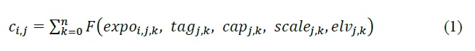
Where each nested vulnerability function is parameterized by the following from the ‘asset inventory (finv)’ (Section4.1):

• tag: variable linking the asset to the corresponding vulnerability curve in the vulnerability curve set (‘curves’);

• cap: maximum value cap placed on the vulnerability curve result;

• scale: scale value applied to the vulnerability curve result;

• elv: vertical distance from the exposure value;

the following from the ‘exposure dataset (expos)’:

• expo: magnitude of flood exposure sampled at the asset.

and the following optional parameter from the ‘control file’:

• curve_deviation:which curve deviation to use.

The ‘Impacts (L2)’ routine first calculates the impacts of each nested function, then scales the values, then caps the values, before combining all the nested values to obtain the total impact for a given asset.

Generally, the exposure dataset (‘expos’) is constructed with the ‘Hazard Sampler’ (Section5.1.3) tool and contains a set of sampled WSL for each asset and each event. However, the only requirements on the ‘expos’ file are that it matches the expectations of the vulnerability functions referenced by the ‘curves’ parameter (Section4.3).

Ground Water

To improve performance, Impacts (L2) only evaluates assets with positive depths (when ‘ground_water’=False) and real depths. By specifying ‘ground_water’= True , negative depths (within the minimum depth found in all loaded damage functions) can be included in the calculation.

Object Level Mitigation Measures

The ‘Impacts (L2)’ model facilitates the modelling of exposure reductions brought about by object (or property) level mitigation measures (PLPM) such as backflow valves or sandbagging. The real effect of such interventions on the hydraulic exposure of buildings or property is complex and may be influenced by: 1) active vs. passive nature of the PLPM; 2) the warning time and time of day or year (for active PLPMs); 3) hydraulic loading on the PLPM; 4) quality of installation of PLPM; 5) operator experience or error (for active PLPMs); 6) maintenance of the PLPM. CanFlood does not consider this complexity; instead, CanFlood facilitates the user’s approximation through simple thresholds, scale factors, and addition values. This parameterization should be provided for each asset in the inventory vector layer (‘finv’) with Section5.2.2 the following fields:

• Lower threshold (mi_Lthresh): All depths below this will generate an impact value of zero.

• Upper threshold (mi_Uthresh): All depths above this will NOT have impact scale factors or impact addition values applied.

• Impact scale factor (mi_iScale): For depths below the ‘upper threshold’, impact values will be scaled by this factor.

• Impact addition value (mi_ iVal): For depths below the ‘upper threshold’, impact values will have this value added to them.

Additional Outputs

For advanced analysis, users can select the ‘dmgs_expnd’ option to output the complete impacts calculated on each nested function of each asset. This large, intermediate, data file provides the raw, scaled, capped, and resolved (The ‘capped’ values with null and rounding treatment) impact values for each asset and each nested function. This can be useful for additional data analysis and troubleshooting but does not need to be output for any model routines (i.e., it is provided for information only).

Another optional output is supplied through the ‘bdmg_smry’ function and corresponding parameter that summarizes the results of each step or routine in the ‘Impacts (L2)’ module. The first tab in the spreadsheet, ‘_smry’, shows the total impacts for each event at each routine in the module. The next group of tabs summarize the impacts calculated on each ftag for the corresponding routine (e.g., ‘raw’, ‘scaled’, ‘capped’, ‘dmg’, ‘mi_Lthresh’, ‘mi_iScale’, ‘mi_iVal’). Two additional tabs are provided to summarize the calculations of the capping routine (i.e., ‘cap_cnts’ and ‘cap_data’).

5.2.3. Risk (L2)

CanFlood’s ‘Risk (L2)’ tool is designed to perform a ‘classic’ object-based deterministic flood risk assessment using impact estimates and probabilities to calculate an annualized risk metric. Beyond this classical risk model, ‘Risk (L2)’ also facilitates risk estimates that incorporate conditional hazard events, like levee failure during a 100-yr flood. This can be conceptualized with Sayers (2012)’s ‘source-pathway-receptor’ framework as shown in Figure5-3, where:

• Source: WSL prediction (in raster format) for levels behind the defense (e.g. levee) of an event with a quantified likelihood.

• Pathway: The infrastructure element separating receptors (i.e. assets) from the raw WSL prediction. Typically, this is a levee, but could be any element where ‘failure’ likelihood and WSL can be quantified (e.g. stormwater outfall gates, stormwater pumps).

• Receptor: Assets vulnerable to flooding where location and relevant variables are catalogued in the inventory and vulnerability is quantified with a depth-damage function.

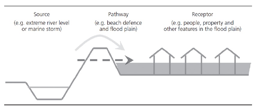
Figure 5-3: Sayers (2012)’s Source-Path-Receptor framework.

Model package requirements for the Risk (L2) tool are summarized in the following table:

Table 5-10: Risk (L2) model package requirements.

Name	Description	Build Tool	Code	Reqd.
Control File	Data file paths and parameters	Start Control File		yes
Event Probabilities	Probability of each hazard event	Event Variables	evals	yes
Exposure Probabilities	Conditional probability of each asset realizing the failure raster	Conditional P	exlikes	for failure
Total impacts	Output of Impacts (L2) model	N/A	dmgs	yes

Outputs provided by this tool are summarized in Table5-7.

Events without Failure

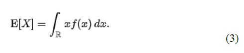
A simple application of the ‘Risk (L2)’ model is a study area with no significant flood protection infrastructure (e.g., a floodplain with no levees), like in Tutorial 2a (Section6.2). In this case, each hazard event has a single probability and a single raster and the results from the ‘Impacts (L2)’ tool simply need to be integrated to yield the annualized risk metric. The primary risk metric calculated by CanFlood is the expected value of flood impacts E[X] (also called Expected Annual Damages (EAD), or Average Annual Damages (AAD), or Annualized Loss) and is defined for discrete events as:

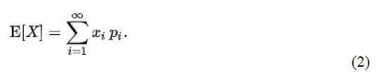
Where x _i is the total impact of the event i and p _i is the probability of that event occurring. While flood models discretize events out of necessity (e.g., 100yr, 200yr), real floods generate continuous hazard variables (e.g., 100 – 200yr). Therefore, the continuous form of the previous equation is required:

Where f(x) is a function describing the probability of any event x (i.e., the probability density function) (USACE 1996). To align with typical discharge-likelihood expressions common in flood hazard analysis, the previous equation is manipulated further to:

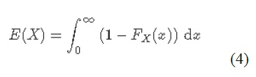
Where Fx(x) is the cumulative probability of any event x (e.g. cumulative distribution function). Recognizing that the complement of Fx(x) is the annual exceedance probability (AEP) (the probability of realizing an event of magnitude x or larger), this equation yields the classic ‘Risk Curve’ common in flood risk assessments shown in Figure5-4.

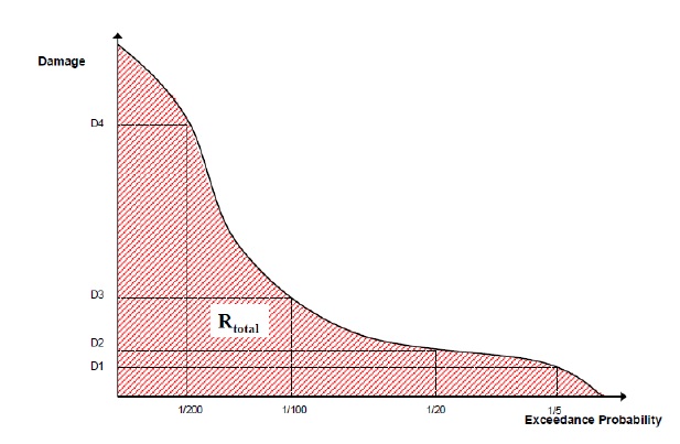
Figure 5-4: Damage-probability Curve from Messner (2007).

The following algorithm is implemented in CanFlood’s ‘Risk (L1)’ and ‘Risk (L2)’ models to calculate expected value:

1. Assemble a series of AEPs and total impacts for each event;

2. Extrapolate this series with the user provided extrapolation handles (‘rtail’, and ‘ltail’);

3. Use the numpy integration method specified by the user to calculate the area under the series.

The same algorithm is used for calculating the total expected value across all assets and for the expected value of individual assets (if ‘res_per_asset’=True).

Events with Failure

When resolving a hazard event with some failure, CanFlood combines the expected value (E(X)) of each companion failure event with that of a base ‘no-fail’ event to obtain the event’s total expected value required by the risk metric equation (formula 4). To provide flexibility in the data requirements from a defense reliability analysis, CanFlood distinguishes two failure event analysis dimensions based on the geometry of the provided conditional exposure probability polygons (‘failure polygons’) and the number of failure events as summarized in Figure5-5. ‘Failure polygons’ complexity is discussed in Section5.1.5 and is resolved into the resolved exposure probabilities (‘exlikes’) dataset by calculating a single exposure probability for each companion failure event (Figure5-5 ‘b1’ and ‘b2’ into ‘f1’). Once simplified into this resolved exposure probabilities (‘exlikes’) dataset, a failure event’s failure polygons set relation, count, and complexity is ignored.

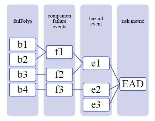
Figure 5-5: Example diagram showing three hazard events, one without failure (e3), one with simple (e2) and one with complex failure events (e1), and two companion failure events with simple (f2, f3) and the other (f1) with complex conditional exposure probability polygons (failure polygons).

Table5-11 summarizes the treatment of hazard events based on the count of failure events assigned to each.

Table 5-11: Hazard event treatment by failure event count.

Type	Count	Treatment 1	Example (Figure5-5)
trivial	0	E(X)fail=0 E(X)nofail from equation 2	e3
simple	1	‘max’ or ‘mutEx’	e2
complex	>1	‘max’, ‘mutEx’ or ‘indep’	e1
See Table5-12

Events with Complex Failure

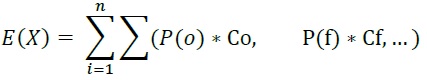
Table5-12 summarize the algorithms implemented in CanFlood to calculate expected value for those hazard events with more than one companion failure event i.e., ‘complex’ failure events.

Table5-12: Expected value algorithms for failure events.

name	Count	summary
Modified Maximum	max
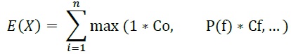
Mutually Exclusive	mutEx
Independent	indep	Construct a matrix of all possible failure event combinations (positives=1 and negatives=0) Substitute matrix values with P and (1-P) Multiply the set to obtain the probability of the combination (P comb) Multiply P comb by the maximum impact of events within the set to obtain the combination’s impact (C comb)
P(o) = 1-sum(C i)

5.2.4. Risk (L3)

Bryant (2019) developed the Stochastic Object-based Flood damage Dynamic Assessment model framework (SOFDA) to simulate flood risk over time using the Alberta Curves and a residential re-development forecast. Framework development was motivated by a desire to quantify the benefits of Flood Hazard Regulations (FHRs) and to help incorporate the dynamics of risk into decision-making. SOFDA quantifies flood risk of an asset through the use of direct-damage and depth-likelihood functions. In this way, flood risk can be quantified (e.g. monetized) at fine spatial resolutions for robust decision support.

SOFDA has the following capabilities:

• Estimate the vulnerability reduction of Flood Hazard Regulations;

• Estimate the vulnerability reduction of Property Level Protection Measures;

• Estimate the influence of elevating damage-features (e.g., raising water heaters);

• Simulate changes in relevant building typology brought about by re-development (e.g., larger homes with deeper basements);

• Dynamic and flexible modeling of many model components (e.g., more expensive water heaters);

• Provide some quantification of uncertainty (i.e., stochastic modeling);

• Provide detailed outputs to facilitate the analysis of underlying mechanisms.

For additional information and guidance, see Appendix B.

5.3. Results

The ‘Results’ toolset is a collection of tools to assist the user in performing secondary data analysis and visualization on CanFlood models. The remainder of this section describes the function of the tools within this toolset.

5.3.1. Join Geo

This tab provides a tool to join the non-spatial risk results back onto the inventory geometry for spatial post-processing. A basic version of this tool can be run automatically by the ‘Risk (L1)’ and ‘Risk (L2)’ tools. On the ‘Join Geo’ tab, the user can perform additional customization of these layers, including applying pre-packaged layer styles.

5.3.2. Risk Plot

This tab contains multiple tools for generating non-spatial plots on a single model scenario. The plots generated on this tab all pull style information from the Control File’s ‘[plotting]’ group, and results data from the ‘[results_fp]’ group. Plots are available in the two standard risk curve formats:

• ARI vs. Impacts

• Impacts vs. AEP

See Section6.3.3 for examples.

Plot Total

This tool generates a simple plot of the total results. A basic version of this tool can be run automatically from the ‘Risk (L1)’ and ‘Risk (L2)’ tools for convenience.

Plot Stack

This tool generates risk curves showing the total contributions from each composite vulnerability functions discussed in Section4.1 on a single plot.

Plot Fail Split

This tool generates composite risk curve showing the total results with a second curve showing the contribution from the ‘non-failure’ portion of each event (i.e., subtracting any contributions from companion failure events) on a single plot.

5.3.3. Compare/Combine

This tab provides two tools for combining or comparing multiple CanFlood models within a single analysis. For example, a flood risk analysis considering agricultural losses and residential building damages would generally construct two separate models (i.e., separate control files) and combine the results at the end to understand the total risk. Alternatively, an analysis may wish to compare two mitigation alternatives.

Compare

The compare tool collects the total results dataset (‘r_ttl’) and parameters from the set of specified control files and produces two comparison outputs:

• Control file comparison: generates a datafile populated with the parameters from each selected control file, and a final column indicating if the parameter varies across the set. This can be useful to indicate what separates two CanFlood models.

• Plot comparison: creates a risk curve plot comparing the total results data set (‘r_ttl’) of all selected control files. Default plot values are taken from the control file specified on the ‘Setup’ tab.

Combine

The combine tool collects the total results dataset (‘r_ttl’) and parameters from the main control file (from the ‘Setup’ tab) to generate two types of outputs:

• Composite scenario: Select this option when running the ‘Combine’ tool to generate a new composite control file and ‘r_ttl’ results file for further analysis.

• Plot combine: creates a stacked risk curve showing the contribution towards the total risk of each selected control file.

5.3.4. Benefit-Cost Analysis

This tab provides two tools to support basic benefit-cost calculations commonly used in flood mitigation options assessments. Benefit-cost analysis (BCA) is a complex process discussed elsewhere (Merz et al. 2010; Smith et al. 2016; IWR and USACE 2017) that carries many challenges and short-comings when applied to decisions around flood mitigation (O’Connell and O’Donnell 2014; Hosein 2016). In short, BCA compares the net-present value of an intervention’s costs (e.g., construction, maintenance) to the benefit or flood-loss avoidance gained by the intervention. Through the application of a discounting rate in these net-present value calculations, BCA are sensitive to the timing or accrual of benefits and costs. A typical workflow in CanFlood implementing BCA is provided below:

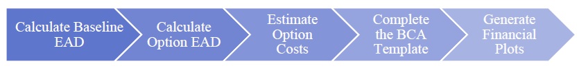
To support simple BCA calculations, CanFlood’s ‘BCA’ tab provides the following tools:

Copy BCA Template

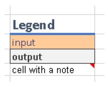
This tool copies the CanFlood BCA template (‘cf_bca_template_01.xlsx’, see below), which has a ‘smry’ and ‘data’ tab, and populates the ‘smry’ tab with metadata from the main control file. This .xlsx file provides a generic template for inputting project cost and benefit time series and calculating summary financial values, like benefit-cost ratio, using EXCEL’s built-in formulas. The workbook contains excel ‘notes’ and implements the following styles to guide users when completing the template:

A portion of the ‘data’ tab is provided below. Users should populate the input cells using the development, operating, and flood loss avoidance values for the option under consideration. Key cells on the ‘input’ tab are ‘named’ to facilitate populating the data tab dynamically.

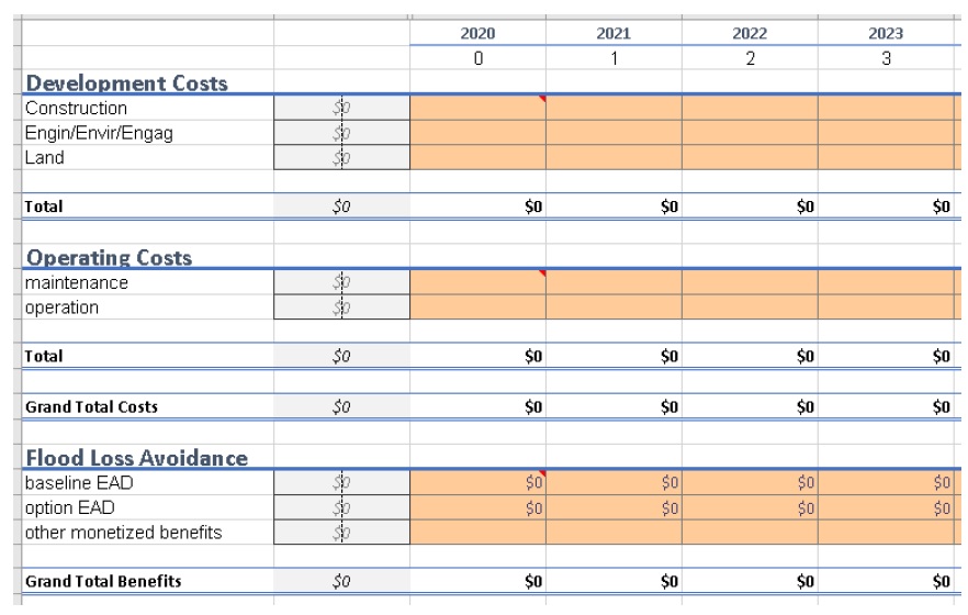
Figure 5-6: CanFlood BCA template ‘data’ tab.

Once the ‘data’ tab is complete, enter an appropriate ‘discount rate’ should be entered on the ‘smry’ tab. Positive discounting rates are commonly used in financial analysis to reflect the view that things of value (e.g., capital) are worth more today than in the future. This should not be confused with inflation. The application of positive discounting rates is inappropriate when evaluating assets with increasing scarcity, like ecosystem function and wild spaces. Some authors and guidelines propose variable discounting rates (Smith et al. 2016). Guidance on selecting an appropriate discounting rate is provided elsewhere (Farber 2016).

After populating the ‘data’ and ‘smry’ tabs, the workbook should display the results summarized below:

PV benefits $

Present Value of benefit totals

PV costs $

Present value of cost totals

NPV $

Net-present value of costs and benefits

B/C ratio

Ratio of PV benefits over PV costs

Plot Financials

This tool generates a financial time-series plot of the benefit and cost data contained in the BCA worksheet.

5.4. Additional Tools

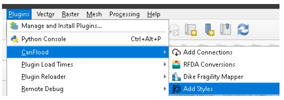
The following section describes some additional tools provided in the CanFlood platform that support flood risk modelling in Canada. These can be accessed from the CanFlood menu (Plugins > CanFlood).

5.4.1. Dike Fragility Mapper

For risk models that incorporate dike defense failure, a dataset containing the conditional probabilities of each asset realizing the failure, called the resolved exposure probability (‘exlikes’) dataset, is required by the Risk (L1) and Risk (L2) modules. Generally, this dataset is generated from a set of ‘failure polygons’ using the ‘Conditional P’ tool in the build toolset (Section5.1.5). While some projects may have these ‘failure polygons’ available, often only event rasters and the dike information discussed in Section4.5 is available. For cases like this, the workflow summarized in Figure5-7 can be employed, beginning with the ‘Dike Fragility Mapper’ tool which provides a collection of algorithms that can be used to generate failure polygons from typical dike information.

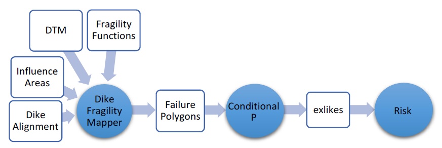
Figure 5-7: Typical CanFlood tools workflow, incorporating dike fragility, where the ‘Dike Fragility Mapper’ tool is used to develop the failure polygons data layer.

The ‘Dike Fragility Mapper’ tool is similar in many ways to the Impacts (L2) module applied to assets with linear geometry, but with the addition of special offset raster sampling, intelligent joining of the results to polygons, and segmentation considerations specific to dike analysis. This tool is executed in the three steps summarized below. For more information on applying this tool, see Tutorial 6a (Section6.11).

Dike Exposure

The dike exposure sub-tool determines the location of highest vulnerability on each dike segment, then returns the corresponding freeboard value of each event raster yielding the dike segment exposure (‘dexpo’) dataset. This is accomplished with the following sequence:

1. Generate transects at specified intervals on specified side of each dike segment (red lines on Figure5-8);

2. Sample the dike crest elevation from the DTM raster at the head of each transect;

3. Sample each event WSL raster on each transect;

4. Calculate the freeboard values on each transect as the difference between the sampled WSL and crest elevation values;

5. Calculate the segment freeboard value by applying the summary statistic to the relevant transect values (default is the minimum value).

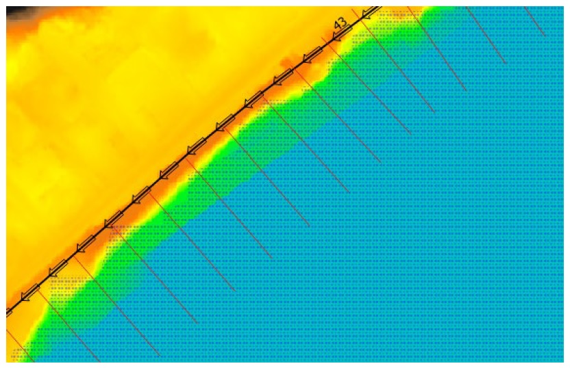
Figure 5-8: Example algorithm components for the Dike Fragility Mapper tool’s exposure routine

This sub-tool provides the following outputs:

• dike segment exposure (‘dexpo’) dataset: freeboard .csv output and main input to the Dike Vulnerability sub-tool;

• processed dikes layer (optional): this is a modified version of the original input file, showing the ‘dexpo’ data on the original dikes geometry;

• transects layer (optional): these are the perpendicular segments of length and spacing specified by the user where the crest elevation and WSL sampling are performed at the head and tail respectively;

• transect exposure points (optional): each transect head with all calculated values;

• breach points layer (optional): transect heads with negative freeboard values;

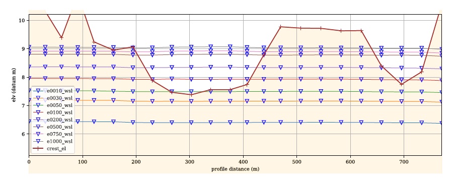
• dike segment profile plots (optional): profile plot of dike segment showing sampled crest elevations and WSL (see below).

Dike Vulnerability

The ‘Dike Vulnerability’ sub-tool feeds the relevant entry in the dike segment exposure (‘dexpo’) dataset into the fragility curve associated with each dike segment. This sub-tool outputs tabular failure probability data (‘pfail’) csv file.

The following algorithms are available to adjust the resulting failure probabilities for the ‘length effect’:

• URS (2008): normalize all failure probabilities by the set of segment lengths.

A similar secondary output is provided for these length-adjusted values.

Dike Failure Probability Results Join

This tool simply joins the selected tabular failure probability data to provided dike influence polygons to generate the ‘failure polygons’ required by the ‘Conditional P’ tool (Section5.1.5).

Notes and Considerations

When applying the Dike Fragility Mapper to your project, the following should be considered:

• CanFlood does not perform any hydraulic analysis, the user must supply influence polygons denoting the area over which assets should have their probability of realizing the corresponding failure raster WSL. Considering this, influence polygons can safely extend beyond the raster extents without affecting the calculation of failure impacts.

• Fragility functions should be developed and tagged to each raster segment by a qualified geotechnical expert using field data.

5.4.2. Add Connections

CanFlood’s ‘Add Connections’ tool adds a pre-compiled set of web-resources to a user’s QGIS profile for easy access and configuration (i.e., adding credentials). The set of web-resources added by this tool are configured in the ‘canflood_parsWebConnections.ini’ file (in the user’s plugin directory). Appendix A summarizes the web-connections added by this tool.

The QGIS User Guide explains how to manage and access these connections. Once the resources are added to a user’s profile, two basic methods can be used to add the data to the project:

• Browser Panel: This is the simplest method but does not support any refinement of the data request. On the Browser Panel, expand the provider type of interest (e.g., ArcGisFeatureServer) > expand the connection of interest > select the layer of interest > right click > Add Layer To Project.

• Data Source Manager: This is the recommended method as it provides more versatility when adding from data connections. Open the Data Source Manager (Ctrl + L) > select the provider type of interest > select the server of interest > select the layer of interest > specify any additional request parameters > click ‘Add’ to load the layer in the project.

Many plugins and tools used by QGIS (and CanFlood) do not support such web-layers (esp. rasters), so conversion and download may be required.

5.4.3. RFDA Converter

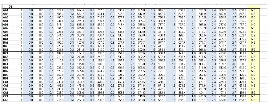
The Rapid Flood Damage Assessment (RFDA) tool was developed by the Province of Alberta in 2014 as a QGIS 2 plugin. RFDA did not include any spatial analysis or risk calculations. RFDA inventories are in Excel spreadsheet format (.xls) indexed by column location (not labels). Curves are tagged to assets using a concatenation of columns 11 and 12. Many columns in the inventory are ignored in RFDA. These are the functional columns:

• 0:’id1’,

• 10:’class’,

• 11:’struct_type’,

• 13:’area’,

• 18:’bsmt_f’,

• 19:’ff_height’,

• 20:’lon’,*

• 21:’lat’,*

• 25:’gel’

*not used by RFDA, but necessary for spatial analysis.

RFDA uses a legacy format for reading damage functions based on alternating column locations. An example is provided below:

RFDA was developed in parallel with a set of 1D damage functions from building surveys of structures in Edmonton and Calgary, AB in 2014. Curves for building replacement/repair and contents damage were developed separately. Residential curves for main floor and basement were developed separately.

During a model run, RFDA applies a contents and structural curve to each asset, and the corresponding basement pair to those with ‘bsmt_f’=True.

To facilitate converting from RFDA inventories to CanFlood format, two tools are provided:

1. Inventory converter; and

2. Damage Curve converter.

Inventory Conversion

The RFDA Inventory Conversion requires a point vector layer as an input (Can be built from an .xls file by exporting to csv then creating a csv layer in QGIS from the lat/long values). For Residential Inventories (those with struct_type not beginning with ‘S’), each asset is assigned a f0_tag with an ‘_M’ suffix to denote this as a main floor curve (e.g. BD_M) based on the concatenated ‘class’ and ‘struct_type’ values in the inventory. Using the ‘bsmt_f’ value, the f1_tag is also assigned with a ‘_B’ suffix. These suffixes correspond to the curve naming of the DamageCurves tool (described below). The f1_elv is assigned from: f0_elv – bsmt_ht.

For Commercial Inventories (those with struct_type beginning with ‘S’), the f0_tag and f1_tag fields are populated with the ‘struct_type’ and ‘class’ values separately. Where ‘bsmt_f’ = True, a third f2_tag=’ nrpUgPark’ is added to denote the presence of underground parking (A corresponding simple $/m2 curve is created by the DamageCurves Converter). Once converted, the user can start the CanFlood model building process.

DamageCurves Converter

This tool converts the RFDA format curves into a CanFlood curve set (one curve per tab). The following combinations of RFDA curves are constructed:

• Individual (e.g. main floor contents)

• Floor combined (e.g. main floor structural and contents)

• Type combined (e.g. structural basement and mainfloor)

• All combined

This allows the user to customize which curves are applied and how to each asset (with CanFlood’s ‘composite vulnerability function’ feature).

5.4.4. Add Styles

To augment the symbol styles packed in QGIS for modifying the display of vector layer features, CanFlood includes a small library of styles typical for GIS flood projects. This library is an .xml file in the plugin directory, and can be added to your style manager through the CanFlood menu as shown below:

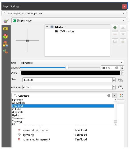
Once executed, these symbols should be available for styling relevant vector layers through one of the QGIS layer styling dialogs. For example, the ‘CanFlood’ group can be accessed via the ‘Layer Styling’ pane (F7) as shown below:

The QGIS ‘Styling Manager’ provides an interface for organizing and other tasks related to styles.

5.4.5. Sensitivity Analysis

CanFlood’s Sensitivity Analysis dialog provides a workflow and tools for performing sensitivity analysis on a L1 or L2 CanFlood model. This can be helpful in understanding and communicating the uncertainty in your model, as well as help identify which parameters should be prioritized during data collection. To use this toolset, the user must first provide a ‘base’ model from which to perform the analysis on. From this base model, the Sensitivity Analysis toolset can be used to: 1) construct a suite of candidate models, where each candidate has a single parameter or dataFile perturbation; 2) run the new model suite; then 3) evaluate the effect of each parameter perturbation on the annualized impact metric (‘ead_tot’).

To facilitate this analysis, the following tabs are provided:

1. Setup the analysis and load the control file

2. Assemble, configure, and compile the candidate model suite

3. Manipulate data files (optional)

4. Run the candidate suite

5. Analyze the results

Compile

This tab provides a tabular readout of the control file parameters for each of your candidate models. To populate the table, first Load a main control file from the Setup tab. Additional candidates can be added and removed using the corresponding buttons. Parameter values can be edited directly in the table; while a convenience method to randomize all the colors is provided (this creates hex color strings readable by matplotlib). It’s a good idea to provide separate colors for each candidate for your later work on the Analysis tab (see below).

To construct each of these candidate models and a working copy of the base model (in their own sub-directory within your working directory), use the Compile Candidates button. This also activates the DataFiles tab and populates the Run tab with each of the compiled control files. Generally, users will want to create separate copies of each datafile (rather than have each candidate point back to the datafiles of the base model) using the ‘Copy all candidate datafiles’ option. This allows the sensitivity of the annualized metric to the data files to be examined by manipulating each duplicated datafile (e.g., adding 1m to all heights). Note using this option will populate the compile table with the new datafile paths, including the paths for the base model. All candidate models use absolute filepaths, regardless of the configuration on the Setup tab.

DataFiles

The DataFiles tab makes it easier to manipulate candidate data files. Once all of the candidates have been compiled (i.e., copied into their own directories), each data file can be accessed through the Candidate Name and Parameter combo boxes. These will populate the data filepath automatically. The datafile can then be loaded into the project (as a memory layer without geometry) from where the fields can be manipulated using the QGIS’s built-in Attribute Table and Field Calculator. Custom expression functions are also pre-loaded under the ‘CanFlood’ menu in the Field Calculator. Once the desired manipulation to the attribute values is applied, the Save Datafile button can be used to write the memory layer back to a csv.

Run

The Run tab displays the control file paths of each candidate model loaded by the Compile Candidates command. This model suite can be run in bulk using the Run button. The results of this bulk-run are stored to a python .pickle file which can be saved for later and loaded in the Analysis tab.

Analysis

The Analysis tab summarizes the outputs from the bulk-run loaded from the python .pickle (see previous section). The table shows some simple statistics, the parameters that were perturbed, and the rank of the candidate model. The rank corresponds to the sensitivity of the annualized metric (ead_tot) to the perturbed parameter, where the rank=1 candidate yielded the largest difference from the base model.

To visualize these values, the PLot Risk Curves button can be used to create a combined risk-curve (similar to the Compare function on the Results toolset). The Plot Box button can be used to create a simple box plot of all the ‘ead_tot’ values.